Unit 7: Rhythm
Synopsis
Rhythm refers to a succession of events in time. While some definitions of rhythm involve concepts like repetition or patterns, psychoacoustics situates these properties in terms of our high level cognition, and studies the processes by which we group and segment streams of events into patterns and phrases. We not only impose patterns on sequences of temporal events, but we are able to recognize these patterns as similar even when they contain substantial temporal variation, making rhythm a potent expressive dimension of music performance. In order to study rhythm, we must be able to say when an event began, and in many cases, this is more difficult than we might expect. For some sounds, particularly those that begin abruptly, the physical onset, that is, the very earliest detection of energy released by the sound source, correlates well with our sense of the perceptual onset, or the moment we associate with the beginning of the sound. For other sounds, however, the physical and perceptual onsets are not the same, making the performance of rhythm, and the study of its performance, significantly more complex than simply playing the right note at the right time.
Rhythm
Introduction
While pitch has received the most attention in perception research, whereas most of music theory consists of putting pitches together to form harmonies, relatively little of common-practice Western musical theory addresses rhythm. Here we define rhythm as the pattern of temporal durations, especially in music. In this unit we will examine the perception and cognition of rhythm. We will begin with the basic observations, e.g. what the optimal range of rhythm and meter are, and how rhythmic subdivisions and expressive timing occur. Then we will discuss the various representations of rhythm, somewhat analogous to visual representations of pitch covered in Unit 5. Finally we will talk about models of rhythm perception and production, and bring in existing literature in an attempt to explain the temporal regularities and deviations that give rise to the human sense of rhythm.
Perceptual Onset Vs Temporal Envelope
It is important to make a distinction between the temporal envelope, the attack portion of which we usually consider to be the beginning of the sound, and the perceptual onset of a sound. In the case of a percussive sound made by a bell or a piano for example, the attack is nearly instantaneous, while other instruments like violins and clarinets have a variety of attacks at their disposal which can make it difficult pinpoint the onset of their sound. Attacks that last less than 30ms tend to sound percussive, while attacks that are longer than 30ms are more like those of a bowed instrument. In the demo called attack-sync, you will hear two sounds, one with a long attack and one with a short percussive attack. When you start the patch, the two sounds will begin together, although, as you will notice, the one with the longer attack will appear to start later. See if you can adjust the start times such that they appear to start isochronously.
(Max patch by Víctor Gutiérrez and John MacCallum)
You can have access to all MUTOR interactive Max patches when you download the maxpatches folder inside the MUTOR github repository and include it in the Max search path.
Subdivision
The optimal range of tempo encoding occurs between 300ms and 1500ms. This is known as the zone of temporal integration, or the tactus. What happens when rhythmic durations are way above tactus? It turns out we subdivide. Subdivision refers to the breaking down of large units into usually even-sized smaller units. In the rhythmic sense the brain is performing chunking, and also building a hierarchical structure of rhythm. As in the frequency dimension for pitch and harmony (see units 5 and 8), small-integer ratios in time play important roles in rhythmic perception. Most rhythmic subdivisions consist of 2:1 ratios, especially in Western music. Rhythms in music of other cultures, e.g. clavé rhythmic patterns in Afro-Cuban and Brazilian rhythms, employ more complex rhythmic patterns, but which can also be broken down into chunks of 2:1 temporal ratios (see Toussaint).
Tactus
Using the demo on synchronous clapping, we may observe that when asked to tap in sync to a rhythmic stimulus, people commonly produce isochronous taps at approximately 1-3 Hz (75-200 taps per minute), i.e. with intervals of approximately 300-800ms between each tap. When the musical stimulus to which we are synchronizing contains sound events below this rate, we tend to subdivide the time by tapping twice per sound event. When the sound to which we are synchronizing is above this rate, we tend to subdivide our tapping by tapping once for every two beats. This optimal rate of rhythmic tapping is called the tactus and is in the range of 300-800ms. The fast end of this range, 300ms or 200 beats per minute, corresponds to the tempo marking of Presto. The slow end, 800ms or 75 beats per minute, corresponds to Adagio. Assuming that our tapping rate reflects our perception of the beat, we can say that the tactus is the optimal range of rhythmic function in music. Several lines of research have addressed why the tactus seems to operate at this range. Some believe that the tactus aids memory: the tactus may reflect the perceptual system’s ability to group distinct sound events together in memory, so that instead of perceiving individual sounds which decay rapidly in sensory memory, we could perceive groups of rhythmic events which hang together to form a Gestalt, or the perception of a whole. Paul Fraisse (from Clarke’s chapter, in Deutsch 1999) believed that the tactus arises from the anatomical constraints of the body and motor functions, as our bodies (musculature, nervous systems, etc) prevents us from tapping at rates faster than 3Hz.
Tatum
In a paper called "A Novel Representation for Rhythmic Structure," Vijay Iyer, Jeff Bilmes, Matt Wright, and David Wessel developed a structure for describing rhythmic events called the tatum (a contraction of temporal atom as well as an homage to the great improvising pianist, Art Tatum). A tatum is a data structure that represents the smallest cognitively meaningful subdivision of the main beat and contains information about it’s probability of occurence, pitch/timbre, accent, duration, and deviation. Musically speaking, a tatum might correspond to 16th notes or 32nd notes in conventional notation, and a measure of music is represented by a vector of tatums. A high probability of occurence means that the beat is likely to be played (after all, not every beat of a bar is played all the time), the accent determines how loudly the beat will be played (this allows for the beginning of the beat of a conventional meter to be accented, for example), the duration vector could either determine the duration of each beat or represent a range of durations from which a random value is chosen, and the deviation allows for the beats to occur slightly early or late and is meant to model the sort of microtiming that human performers inadvertently add to their music and that computers lack.
Accents and Event Stream Vectors
A piece of music is represented by an event-stream vector which contains all of the data for every tatum. An example of a vector representing a bar of 4/4 music might have a set of vectors as represented in table 1.
| Beat | Probability | Accent | Duration | Deviation |
| 1 | 1 | 1 | 1 | .1 |
| 2 | .5 | .25 | 1 | .1 |
| 3 | 1 | .75 | 1 | .1 |
| 4 | .75 | .5 | 1 | .1 |
Table 1.
In 4/4, the first beat is accented the strongest, the third beat the next strongest, the fourth beat is accented slightly as an upbeat to the next bar, and the second beat is the weakest. This is reflected in the probablity of occurence and accent vectors in table 1. The duration in this case is set at 1 which would signify a full beat and the deviation is very low. Table 2 represents a series of tatums that would produce a waltz-like feel.
| Beat | Probability | Accent | Duration | Deviation |
| 1 | 1 | 1 | 1 | 0 |
| 2 | .5 | .25 | .5 | .1 |
| 3 | .75 | .75 | .5 | .1 |
Table 2.
In the above examples, only the main beats of the measures are represented, however, in practice the vectors would contain information about every rhythmic event down to the smallest subdivision.
Microtiming and Expressive Timing
With respect to rhythm, performances of music are often considered cold and lacking in feeling. It is tempting to think that if the metronome marking is 60 BPM, that the 16th-notes should go by at precisely 250 ms. Human performances, however are filled with small deviations in timing, often called microtiming or expressive timing. These small deviations, while not always overtly noticible, contribute to that human feeling that computer performances lack. In the following two examples, you will hear a melody from Robert Schumann’s Träumerei, the first played without expressive timing, while the second includes deviations in timing.
mechanical timing
|
| |
expressive timing
|
| |
(Audio source: Donald Betts. Copyright: Public domain)
(source: Penel & Drake, 2000. Rhythm in music performance and perceived structure. In (Desain et al., 2000)
Above, in the section on the TatuM, along with the parameters of probability of occurence, duration, etc., we also defined a deviation vector. This deviation in timing is meant to mimic the microtiming found in human performance.
Time Maps
Time maps are visual representations of rhythm and meter. These are useful because they help us visualize, analyze, and understand the black box of each individual performance by each musician.
Two kinds of time maps we introduce here are the rhythmogram and the maps of performance time as a function of score time. These two time maps are drastically different and are useful in different applications. The rhythmogram is a time map of event frequencies of notes, which enables the inference of the hierarchical rhythmic structure of a musical piece. The maps of score time versus performance time allow for a coherent representation of the entire performance of a piece; they effectively capture the characteristic expressive deviations of each performer.
In addition to the rhythmogram and the score vs performance time map, various other rhythmic representations deserve mention. Desain and Honing describe a triangular space called the chronotopic map that represents all possible expressive deviations given a four-note rhythm.
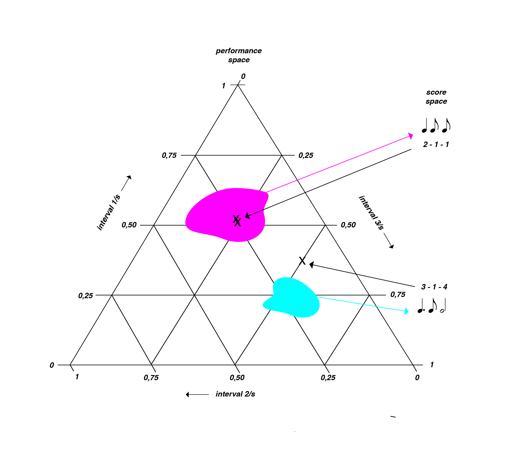
(Image by Janina Luckow. Adapted from: (Desain et al., 2003) Perception.)
Other statistical methods to analyze rhythm and expressive microtiming are also widely used. Benadon uses histograms, which are graphs plotting the occurrence frequencies of events, to diagram the beat-upbeat ratios (BURs) of the swing rhythm in jazz. (Benadon, 2006)
Score Time Vs Performance Time
Given the discussion of microtiming above, it should be clear by now that there is not necessarily a 1:1 correlation between the printed score and what a performer plays. A simple score may only contain pitches, rhythms, some dynamics, and information about the tempo and meter. Although it may lack direction about how to vary the timing expressively, we are not necessarily meant to interpret that lack of direction as an indication that we should play the music as straight and precisely as possible. When directions are given, they are often vague at best, as in the term rubato. As we mentioned above, a computer simulation that lacks microtiming and is based only on what we might call score time tends to feel cold and mechanical. We can begin to understand what a performer brings to the piece with respect to expressive timing by plotting the score time against the performance time as in figure 1.
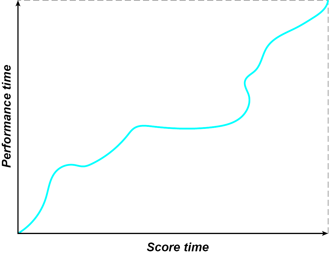
(Image by James Cheung)
By modelling the relationship between score and performance time, one can create a synthesizer that will play music with a more human feel (A Novel Representation for Rhythmic Structure).
Rhythmogram
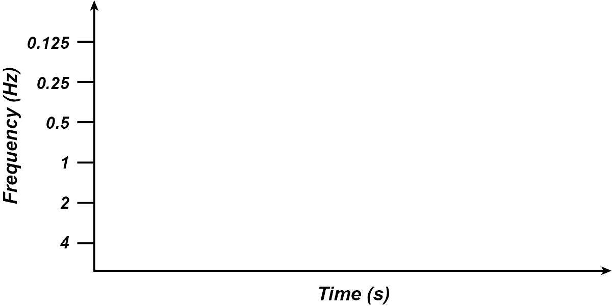
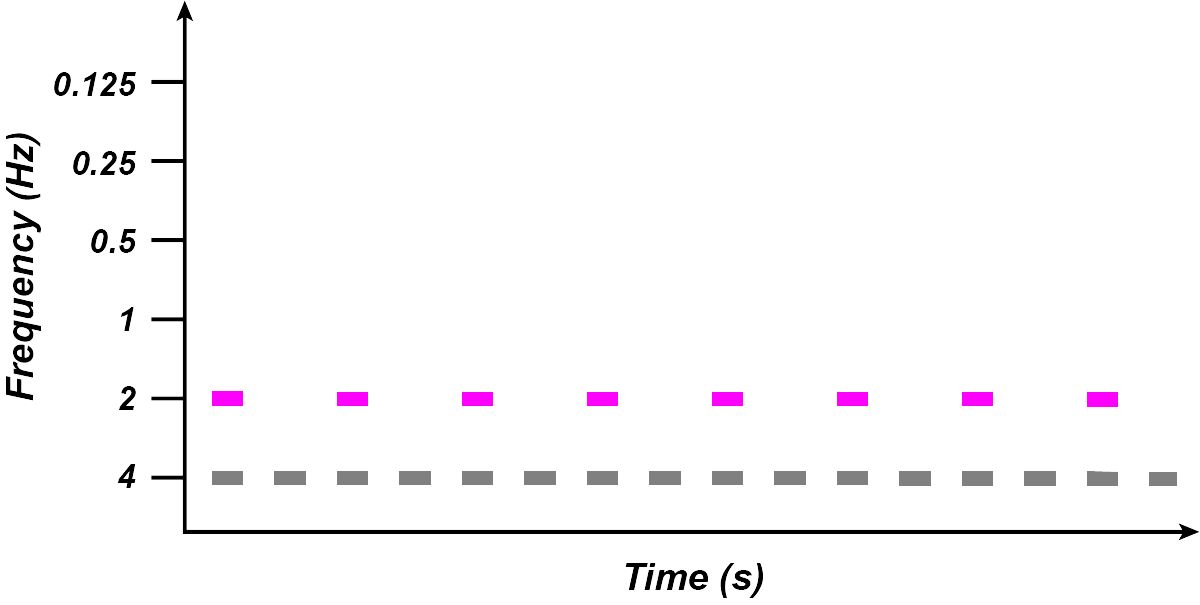
The rhythmogram is an effective way to visualize rhythmic structure in a musical score or performance. First used by Neil Todd (Todd, 1994) (mentioned in E. Clarke in Deutsch, 1999), the rhythmogram is a graph of musical performances with time on the x axis and a low-frequency filterbank on the y axis.
To visualize the low-frequency filterbank, consider a set of very low-frequency bandpass filters arranged logarithmically. For instance, several filters along the filterbank could be: 0.125Hz, 0.25Hz, 0.5Hz, 1Hz, 2Hz, and 4Hz. The rhythmogram plots musical time on the x axis and these filters on the y axis.
(Image by James Cheung. Adapted from: (Todd, 1994))
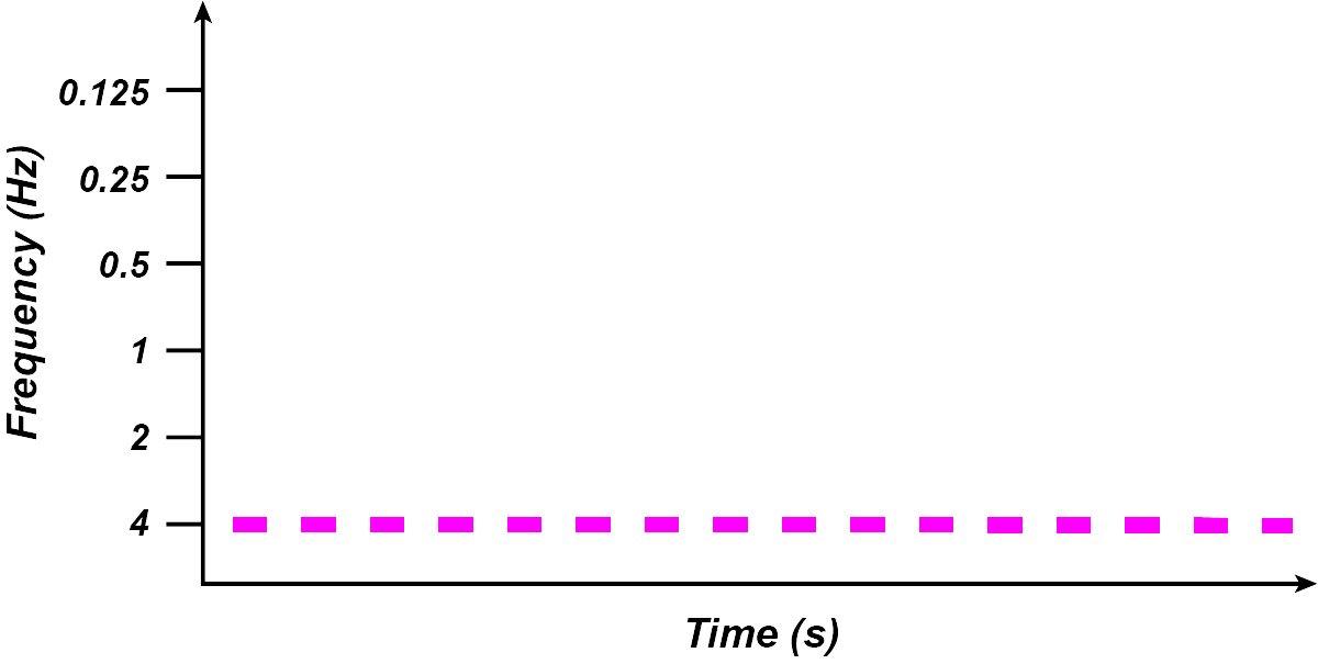
In this representation, notes which occur quickly, e.g. sixteenth notes, would show activity at the highest frequency filters along the filterbank.
(Image by James Cheung. Adapted from: (Todd, 1994))
Notes occurring at the next fastest level, i.e. eighth notes, would appear as activity at the next level of filters:
(Image by James Cheung. Adapted from: (Todd, 1994)) The next level of notes (quarter notes) would then appear energy at 1Hz filters, half notes at 0.5Hz filters, and finally, at the highest level, whole notes would appear at 0.25Hz filters.
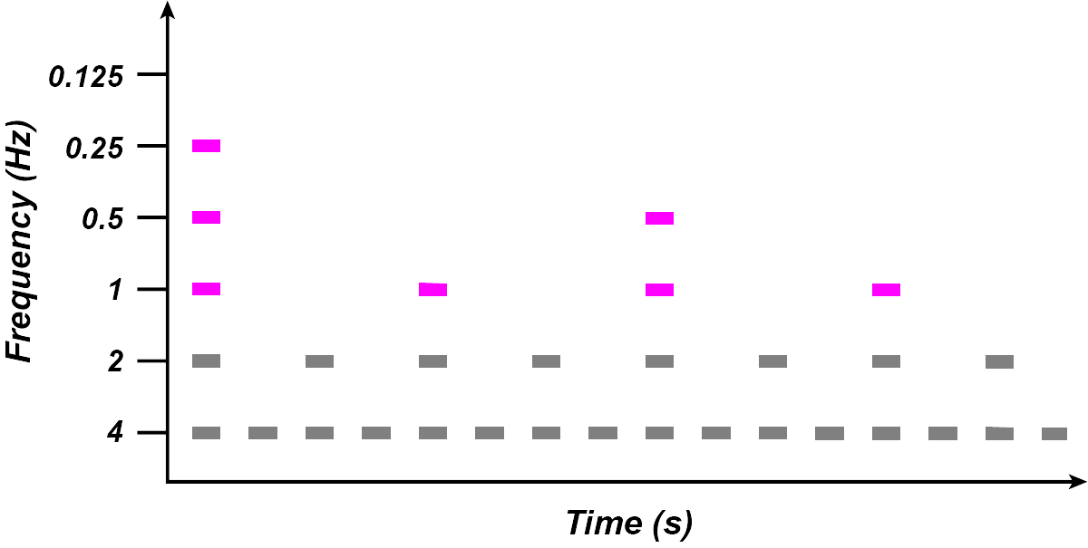
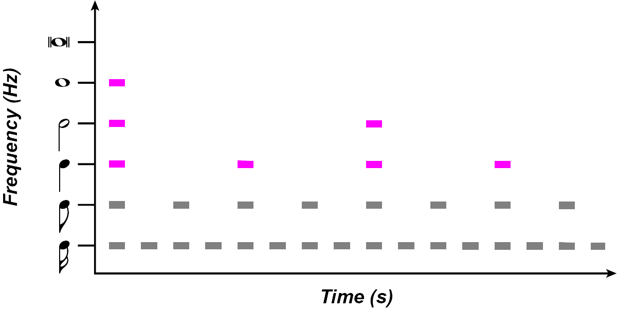
(Image by James Cheung. Adapted from: (Todd, 1994)) Taken together, we see an emergent tree-like diagram of rhythmic activity, with the different layers of the filterbank representing each level of rhythmic structure and importance. Thus, we can say that the rhythmogram provides a visual representation of the tree-like rhythmic structure of a musical piece.
(Image by James Cheung. Adapted from: (Todd, 1994)) The theoretically derived rhythmogram can be applied to actual performances to represent not only the rhythmic structure of the composition, but also the perceptual experience of the piece as a function of its decay rate over time. This links the mathematical idea of a filterbank to the auditory system, with its built-in mechanisms for the detection of onsets. In addition, the rhythmogram could be used to represent the sound structure of speech as well as music.
An application of the rhythmogram to represent perceptual decay is shown here in the speech utterance “tennessee air”:
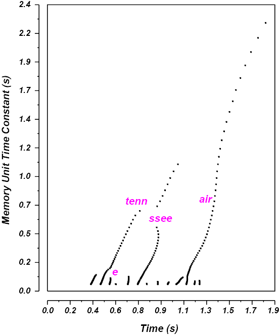
(Image by James Cheung. Adapted from: Todd, 1994)
Instead of a low-frequency filterbank, the above rhythmogram uses a the rate of decay of memory as its y axis. Notes which are more important in the rhythmic structure would be in memory for longer; thus, it would take a higher number of seconds to decay from memory.
This use of the rhythmogram also yields a tree-like structure, which can be represented diagramatically:
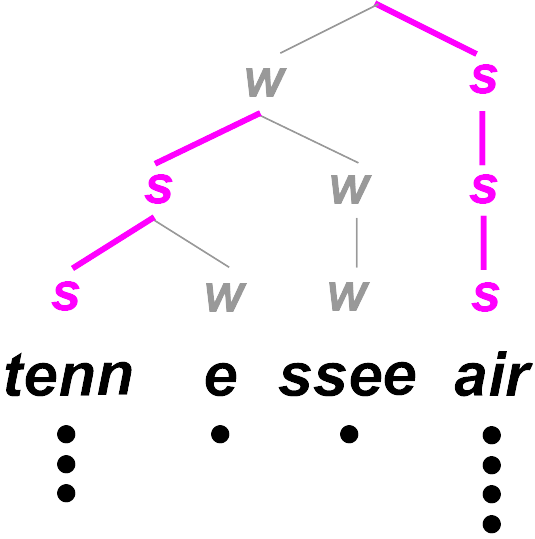
(Image by James Cheung. Adapted from: Todd, 1994)
Using the rhythmogram, the hierarchical structure of music and speech can be derived based on signal processing methods.
Models of Rhythm Perception
Humans seem to have remarkable ability to perceive and produce rhythm. How do we account for such abilities scientifically? What is it about our bodies and our minds that enables the perception and production of rhythm?
Here we present two models of rhythm perception and production: the interval timing model and the coupled oscillator model. The interval timing model predicts the inter-onset interval between two events by viewing Again, it is not clear that the answer must be one or the other; the truth may well lie somewhere in between, or it may be a third model which differs from both interval timing and coupled oscillator models.
An alternate model that relates rhythmic perception and production uses the Bayesian prediction framework, which predicts the probability of an event based on its prior probability, via the BayesRule. This framework has been applied to rhythm to predict rhythm production based on rhythm perception (Sadakata et al., 2006).
Interval Timing
Interval timing models of rhythmic perception and production posit that each rhythmic event is related to its previous event via a pacemaker, or accumulator. The pacemaker is a central timekeeper that sets an overall speed, or tempo, controlling the series of rhythmic events. The accumulator receives pulses from the pacemaker, and compares each interval to the interval immediately before it.
Pacemaker and accumulator models are well supported by neural evidence. Neurological patients with lesions in the basal ganglia, such as patients with Parkinson’s Disease, have trouble keeping time accurately at high levels; that is, they tend to speed up or slow down their tempo significantly over time. In contrast, patients with cerebellar damage have trouble maintaining time at smaller intervals; their timing tends to be uneven and noisy. Taken together, these results suggest that the basal ganglia may act as a pacemaker, or a central timekeeper, whereas the cerebellum acts as an accumulator which corrects each individual rhythmic event by comparing it to its previous event.
Covariance Model
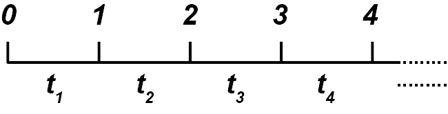
One common observation in rhythm production is that when asked to tap evenly, humans tend to produce rhythms that are slightly uneven. For example, suppose you are required to produce even taps of two taps per second. Here is a time line of your expected taps, in seconds:

(Image by James Cheung)
However, it turns out that the actual measured production is as followed:

(Image by James Cheung)
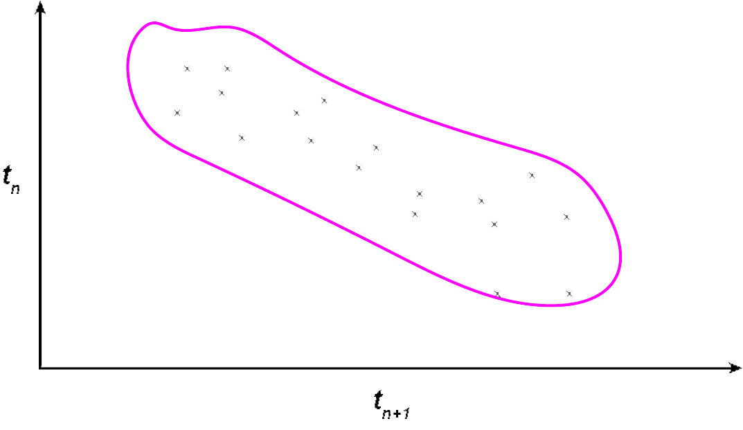
The simplest mathematical model to predict this pattern of behavior is the covariance model. The covariance model proposes that a negative correlation exists between the time interval between two taps and the time interval between the two taps immediately preceding. That is, if $t_n$ is the time interval between successive taps, i.e.
(Image by James Cheung)
Then for every time interval $t_n$, the next time interval, $t_{n+1}$, is negatively correlated in length.
(Image by James Cheung)
If $t_n$ is long, then $t_{n+1}$ is short; if $t_n$ is short, then $t_{n+1}$ is long. (This is the negative correlation principle). Much of the deviations between rhythmic tapping can be modelled this way.
Coupled Oscillator
In contrast to the IntervalTiming models of rhythm, the coupled oscillator models conceive of rhythm as the result of recurring cycles of individual processes known as oscillators. An oscillator is a device which produces a recurrent output at a fixed frequency determined by its own properties, with an amplitude that depends on the amount of energy given to it. A sine wave is a simple output of an oscillator. A spring and a pendulum are both prime examples oscillators.
(Animation by Janina Luckow)
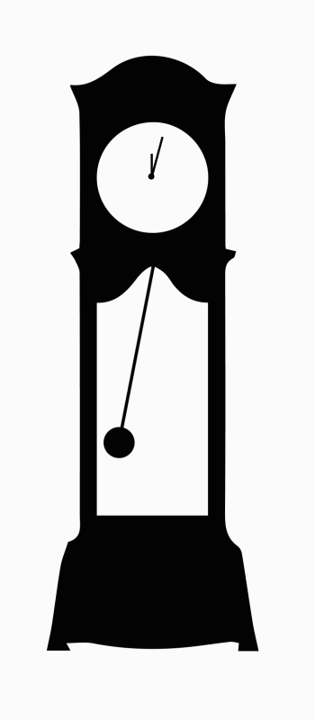
A grandfather clock contains a pendulum, which is a kind of oscillator.

(Animation by Janina Luckow)
A simple pendulum.

(Image source: Martha Takats)
A spring is another example of a simple oscillator.
The coupled oscillator model states that a set of oscillators entrain to each other - that is, their frequencies become tuned to each other, or become coupled as a result of the interaction between two oscillators.

(Image source: Martha Takats)
Coupled oscillators as two symmetrical springs.
Coupled pendulum oscillators

(Animation by Janina Luckow)
Applied to rhythm, the coupled oscillator model states that rhythm is the result of a set of internal oscillators which entrain towards the expected rhythm. Large and Kolen (Large et al., 2007) and McAuley (1996) have modeled the perception and production of rhythm using coupled oscillators, where the placement of each beat within a metric structure is set by the phase of the oscillator, and individual oscillators entrain towards the recurrent beat. The use of coupled oscillators has led to some successful beat-finding algorithms. Coupled oscillator theories are computationally attractive as they can predict many observations, including the perception of meter as a recurrent rhythmic pattern, using relatively elegant mathematical models. Unfortunately, we are not yet sure of physiological bases of coupled oscillator models.
A Mathematical Model of Meter: Clarence Barlow’s Indispensability Function
In Western music, the inherent quality of a meter can be, within limits, encoded by the time signature and the beams employed in its notation. While measures in 3/4, 6/8 and 12/16 meters contain the same number of 16th notes, musicians have learned accentuate the pulses to give them a distinct character. A meter can be considered a kind of relief upon which the gestalt of a rhythm is formed. A rhythm in conjunction with a series of pitches forms the gestalt of a melody (see Unit 8). While a meter conditions a rhythm, syncopated rhythms can go against the grain of the underlying meter.
The composer and music theorist Barlow developed in the 1970s a quantitative model capable of yielding a metric profile for any given meter. Such a profile assigns a unique weight value (indispensability) to each of its pulses. The term indispensability stems from thinning experiments in which Barlow asked subjects to determine which pulses are necessary to maintain a clear sense of a meter when successively turning its pulses into rests and therefore are less dispensible. A metric profile thus represents a kind of “natural order” akin to a harmonic series. But just with the tones derived from the harmonic series, composers and improvising musicians are free decide when and how to violate this order, using this as a means to play with tension and relief on a temporal level.
A meter consists of one to several strata highlighting its hierarchical nature. For example, 6/8 meter is composed of two strata, one with 2 pulses (dotted quarter notes) at the highest level and another with 3 pulses (eighth notes subdividing each of the dotted quarter notes) at the next lower level.
Each stratum is identified by a prime divisor. These are “basic” meters, usually with 2 and 3 pulses; but additive meters such as 5 (2+3) or 7 (2+2+3), can also be defined as basic meters. The indispensability values of a 2 meter are 1 0, those of a 3 meter are 2 0 1, and those of a 5 (2+3) meter are 4 0 3 1 2.
The following meters have the same number of pulses, yet a different stratification yielding the following profiles:
3/4 (3x2x2): 11 0 6 3 9 1 7 4 10 2 8 5
6/8 (2x3x2): 11 0 6 2 8 4 10 1 7 3 9 5
12/16 (2x2x3): 11 0 4 8 2 6 10 1 5 9 3 7
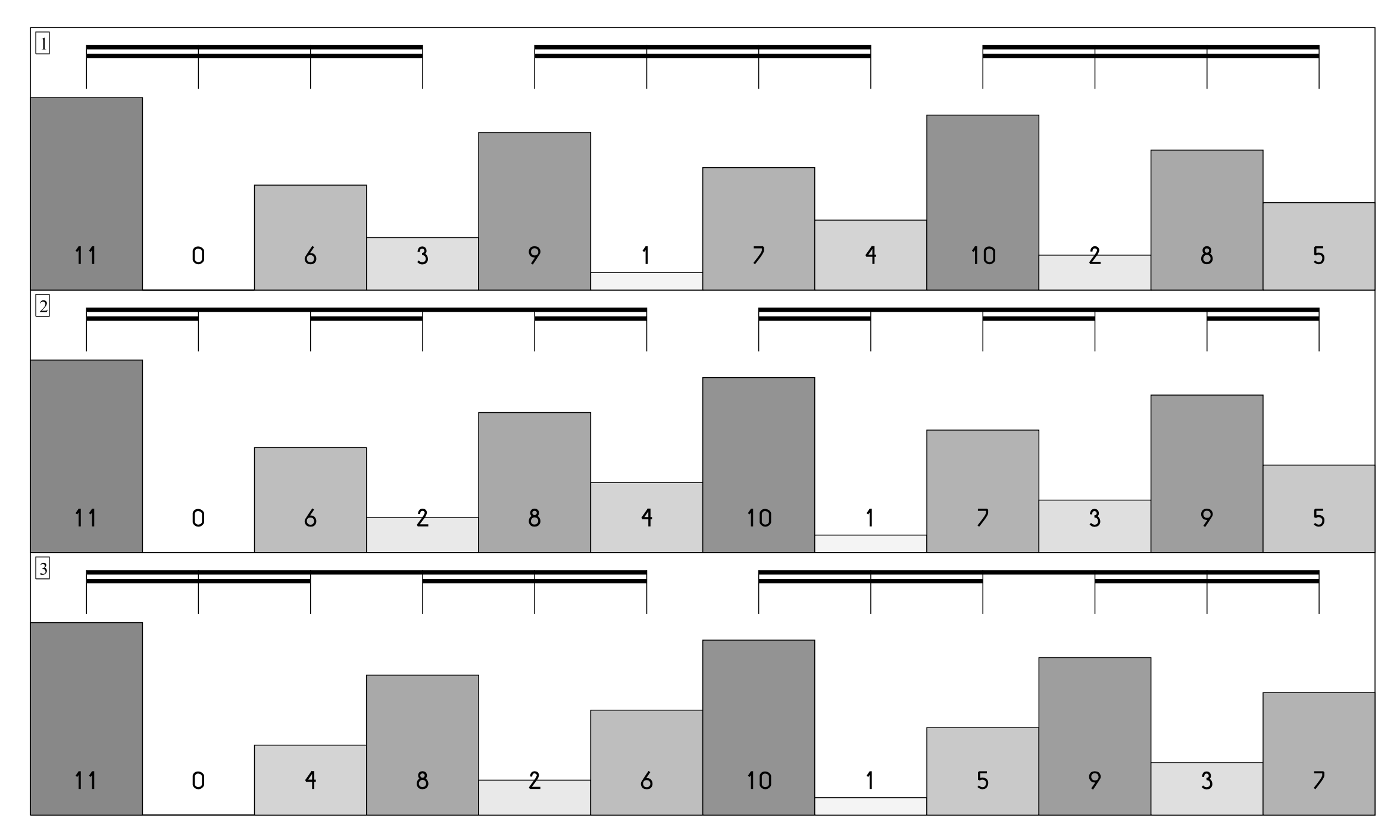
(Image source: (Barlow, 2012))
The values for the first and second levels are also contained herein: to make these evident, subtract the difference between the quantity of pulses at the level shown above and those at the desired level from the indispensability, keeping only non-negative numbers, e.g. for 3/4 (the number of pulses on the 3rd level as shown above is 12):
1st level (pulse quantity 3:subtract 12-3,i.e.9):
2 - - - 0 - - - 1 - - -
2nd level (pulse quantity 6:subtract 12-6,i.e.6):
5 - 0 - 3 - 1 - 4 - 2 -
Note that at all levels, the indispensability of the first pulse is always one less than the number of pulses, and that that of the second pulse is always zero.
The metric profile of a compound meter is obtained by adding the indispensability values of the basic profiles of each strata, rotating the first value backwards in each case.
12/16 meter:
Pulse # 2 3 4 5 6 7 8 9 10 11 12 1
1st stratum 0 0 0 0 0 0 1 1 1 1 1 1
2nd stratum 0 0 0 1 1 1 0 0 0 1 1 1
3rd stratum 0 1 2 0 1 2 0 1 2 0 1 2
Pulse # 2 3 4 5 6 7 8 9 10 11 12 1
*1: 0 0 0 0 0 0 1 1 1 1 1 1
*2: 0 0 0 2 2 2 0 0 0 2 2 2
*2*2: 0 4 8 0 4 8 0 4 8 0 4 8
Sum 0 4 8 2 6 10 1 5 9 3 7 11
Rotating the first pulse back to the beginning yields:
11 0 4 8 2 6 10 1 5 9 3 7
Similarly, for a 2x3x5 meter (e.g. a 6/4 meter with every quarter note further divided by 5 sixteenth-note quintuplets), we initially get:
Pulse #:
2 3 4 5 6 7 8 9 10 11 12 13 14 15 16 17 18 19 20 21 22 23 24 25 26 27 28 29 30 1
1st stratum:
0 0 0 0 0 0 0 0 0 0 0 0 0 0 0 1 1 1 1 1 1 1 1 1 1 1 1 1 1 1
2nd stratum:
0 0 0 0 0 1 1 1 1 1 2 2 2 2 2 0 0 0 0 0 1 1 1 1 1 2 2 2 2 2
3rd stratum:
0 3 1 2 4 0 3 1 2 4 0 3 1 2 4 0 3 1 2 4 0 3 1 2 4 0 3 1 2 4
Now we multiply each stratum by the product of the pulse counts of the preceding strata (1 for the first stratum) and add the values together:
Pulse #:
2 3 4 5 6 7 8 9 10 11 12 13 14 15 16 17 18 19 20 21 22 23 24 25 26 27 28 29 30 1
*1:
0 0 0 0 0 0 0 0 0 0 0 0 0 0 0 1 1 1 1 1 1 1 1 1 1 1 1 1 1 1
*2:
0 0 0 0 0 2 2 2 2 2 4 4 4 4 4 0 0 0 0 0 2 2 2 2 2 4 4 4 4 4
*2*3:
0 18 6 12 24 0 18 6 12 24 0 18 6 12 24 0 18 6 12 24 0 18 6 12 24 0 18 6 12 24
Sum:
0 18 6 12 24 2 20 8 14 26 4 22 10 16 28 1 19 7 13 25 3 21 9 15 27 5 25 11 17 29
Rotating the final number back to the beginning yields:
29 0 18 6 12 24 2 20 8 14 26 4 22 10 16 28 1 19 7 13 25 3 21 9 15 27 5 25 11 17
The following formula by Clarence Barlow formalizes this process (the rotation is applied by the addition of the 1 within the round and square brackets):
\begin{equation} \Psi_z (n) = \sum_{r=0}^{z-1}\left \{ \prod_{i=0}^{z-r-1} p_i \Psi_{p_{z-r}} \left ( 1+\left( \left \lfloor 1+\frac{(n-2)\mod \prod_{j=1}^{z}p_j}{\prod_{k=0}^{r}p_{z+1-k}} \right \rfloor \mod p_{z-r} \right ) \right ) \right \} \label{eq:barlow-indispensibility} \end{equation} Formula of the indispensability $/Psi$ of the $n$th pulse of a meter of stratification $p_1 \times p_2 \times \cdots \times p_z$
whereby
$ p_0 = p_{z+1} = 1 $
$ n = $ position in the bar of the pulse in question, starting at 1
$ p_j = $ stratification divisor on level $j$
$ z = $ number of levels in the stratification
$ \Psi_p (x) = $ indispensability of the $x$th pulse of a first-order bar with the prime stratification $p$
$ \lfloor x \rfloor = $ whole-number component (floor) of $x$.
The indispensability of the 24th pulse ($n=24; z=3$) can thus be calculated:
For $r=0$: $(2\times 3) \times \Psi_5 (1 + \lfloor 1 + \frac {22\mod 30} {1} \rfloor\mod 5) = 6 \times \Psi_5 (1 + 23\mod 5) = 6 \times \Psi_5 (1 + 3) = 6 \times 1 = 6$
For $r=1$: $2 \times \Psi_3 (1 + \lfloor 1 + \frac{22 \mod 30}{5} \rfloor\mod 3) = 2 \times \Psi_3 (1 + 5.4\mod 3) = 2 \times \Psi_3 (1 + 2) = 2 \times 1 = 2$
For $r=2$: $1 \times \Psi_2 (1 + \lfloor 1 + \frac{22 \mod 30}{15} \rfloor\mod 2) = 1 \times \Psi_2 (1 + 2.47\mod 2) = 1 \times \Psi_2 (1 + 0) = 1 \times 1 = 1$
The sum of the three value is therefore 9 (see above).
This formula can be extended to also work with additive meters such 2+3+3+2+3, whereby all segments consisting of number 2 ought to be considered truncated 3 meters. This example derives from a $5\times 3$ meter with two of its groups (first and second to last) truncated, i.e. the missing pulses are removed from the profile and its indispensabilities collapsed in order to avoid gaps:
5x3 meter:
14 0 5 10 3 8 13 1 6 11 2 7 12 4 9
Remove pulses and collapse indispensability values
2+3+3+2+3 meter:
14 0 [5] 10 3 8 13 1 6 11 2 [7] 12 4 9
=>
12 0 8 3 6 11 1 5 9 2 10 4 7
Barlow has often used such profiles in those compositions for which he used a probabilistic generative approach (i.e. weighted chance operations), his 30-minutes piano piece Çoǧluotobüsişletmesi among them.
Summary
We have provided an overview of the physic and biology of rhythm perception and production. Our perception of rhythm depends on sounds; in particular on perceptual accents or event onsets within the streams of sounds to which we are exposed in the environment. Rhythm seems to function optimally at the range of the Tactus, and can be subdivided into the smallest unit known as the Tatum. Microtiming and expressive timing can be described using time maps, which include the rhythmogram and graphs relating score time to performance time. Models of rhythm and meter can be divided into two broad classes known as the interval timing models and the coupled oscillator models. In some cases, rhythm production can also be modeled as covariance. The Bayesian method provides a method to relate rhythm perception with production.
Quiz
What are the important features of sound that enable the perception of rhythmic beats?
What is the optimal range of rhythmic function? How do we know?
What are the axes of a rhythmogram?
What is microtiming?
What are the relative advantages and disadvantages of the interval timing model and the coupled oscillator model?
References
- Toussaint, G. “The geometry of musical rhythm: what makes a "good" rhythm good?”. CRC Press. 2019.
- Iyer, V. “Microstructures of Feel, Macrostructures of Sound: Embodied Cognition in West African and African-American Musics”. Doctoral Dissertation, University of California, Berkeley. 1998.
- Desain, P. & Windsor, L. “Rhythm perception and production”. http://www.nici.ru.nl/mmm/papers/rpp-book/rpp-book.html. 2000.
- Todd, N.P. “The auditory “primal sketch”: A multiscale model of rhythmic grouping”. Journal of New Music Research, 23: 25-70. 1994.
- Benadon, F. “Slicing the beat : Jazz eighth-notes as expressive microrhythm”. Ethnomusicology, 50(1): 73-98. 2006.
- Desain, P. & Honing, H. “The Formation of Rhythmic Categories and Metric Priming”. Perception. 2003. 10.1068/p3370
- Diedrichsen, J. & Ivry, R.B. & Pressing, J. “Cerebellar and basal ganglia contributions to interval timing”. In Functional and neural mechanisms of interval timing, Meck, W.H. (Ed.), pp. 457–483. 2003.
- Sadakata, M. & Desain, P. & Honing, H. “The Bayesian way to relate rhythm perception and production”. Music Perception, 23(3): 267-286. 2006.
- Buhusi, C.V. & Meck, W.H. “What makes us tick? Functional and neural mechanisms of interval timing”. Nature Reviews Neuroscience, 6: 755–765. 2005.
- Large, E.W. & Kolen, J.F. “Resonance and the Perception of Musical Meter”. Connection Science, 6: 177-208. 2007. 10.1080/09540099408915723
- Barlow, C. “On Musiquantics”. Report No.51 of the Musicological Institute / Musikinformatik & Medientechnik of the University of Mainz. 2012.
Authors
Topics
- Introduction
- Perceptual Onset Vs Temporal Envelope
- Subdivision
- Tactus
- Tatum
- Accents and Event Stream Vectors
- Microtiming and Expressive Timing
- Time Maps
- Score Time Vs Performance Time
- Rhythmogram
- Models of Rhythm Perception
- Interval Timing
- Covariance Model
- CoupledOscillator