Unit 6: Timbre

Synopsis

Why does an oboe sound different than a violin? The quality of a sound that helps us make that and other differentiations is called timbre and is notoriously difficult to define, describe, and measure. Although the timbre of a sound may be just as hard to qualify as it is to quantify, its effects on the relationship of one sound to another can profoundly impact our overall experience of them, even strengthening or weakening their structural function in a musical context. To study the timbral characteristics of a sound, we often analyze certain characteristics of its spectrum, such as its envelope, centroid, or noisiness. These measures loosely correlate with many of the ways in which we describe sounds, and help us better understand what it means when we say a sound is “bright” or “dark” or “hollow”, etc. However, the temporal evolution of a sound, particularly in the first few milliseconds before the spectrum stabilizes to some degree, has such a strong impact on the way we perceive the timbre of a sound, that without it, we are often unable to discern the source of an otherwise familiar sound.

• Introduction
• Descriptions of Timbre
• Spectrum
  • Global Features of the Spectrum that Relate to Timbre
    • Spectral Envelope
    • Spectral Centroid
    • Formants
  • Local Features of the Spectrum that Relate to Timbre
    • Even / Odd Balance
    • Harmonicity
    • Proximity of Partials to one Another
      • Sensory Consonance and Dissonance
• Temporal Evolution of the Spectrum
  • Temporal Envelope
  • Onset of Partials
  • Transients
• Timbre and Orchestration
  • Klangfarbenmelodie
  • Timbre Space as a Musical Control Structure
• Quiz
• References

Introduction

Timbre is tricky to define, but we can start with this: all things being equal, i.e. perceived pitch, loudness, etc., timbre is the quality that makes a clarinet sound like a clarinet, a violin sound like a violin, and the two sound different from each other. Timbre can be thought of as the auditory equivalent of color. Timbre itself is not measureable, i.e. it is not an intrinsic property of a sound, but rather, a perceptual one. However, it is related to certain physical charasterics of sound that are measureable, such as the spectrum.

In this unit, we will discuss the physical characteristics of sound that are related to timbre, as well as the role of timbre in the organization of musical structure.

Descriptions of Timbre

Many of our most common terms for describing timbre, e.g. bright, dark, full, rich, thin, piercing, hollow, warm, cold, brittle, velvety, smooth, etc. rely on metaphors that involve senses other than audition. Generally, these terms refer to the distribution of energy in the spectrum and the way in which that energy changes over time. It is this multidimensional nature of timbre, as well as its intersection with both the physical and perceptual world that make it difficult to get a handle on and put into words (Wallmark, 2018).

Spectrum

As we saw in Unit 1, a spectrum represents a complex sound that has been decomposed into a sum of simpler parts, usually sine waves. Pure sine waves have no overtones, and they are the only waveforms without them. All other sounds are complex, that is, they have energy spread across multiple areas of the audible frequency range (roughly 20-20,000 Hz), and the spectral representation of a sound gives us information about how that energy is distributed.

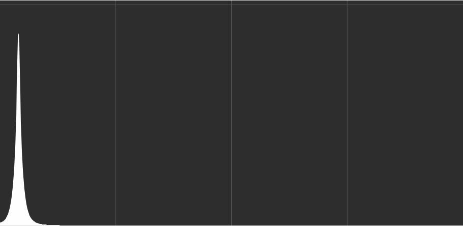
Typically, we look at a spectrum on a 2D plot, like so:

Time-domain representation of a signal.

(Image by John MacCallum)

Frequency-domain representation of a signal.

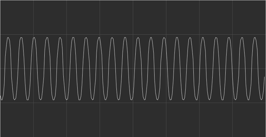
(Image by John MacCallum) In the plot on top, we have a familiar sine wave; the vertical axis represents amplitude, and the time is along the horizontal axis, which is why we refer to this representation as the time-domain. In the bottom plot, the vertical axis is the magnitude (related to the amplitude), and the horizontal axis represents frequency, making this a frequency-domain representation.

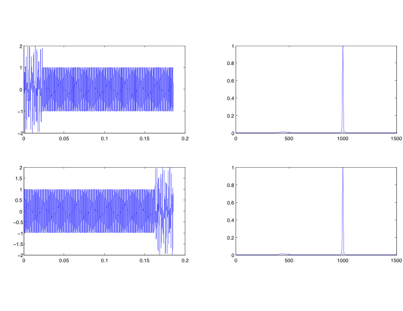
Practically speaking, the spectrum represents an average of the energy distribution over a window of time. The spectrum in the bottom plot above was made from the entire signal above it. Because it is an average taken over a period of time, temporal events that happen within that span of time contribute to the average, but can only be said to have occurred within the span—we cannot say where exactly they occurred. This can be seen clearly in the figure below, in which two time-domain waveforms, one with an event at the beginning, and the other with an event at the end, produce the same spectra.

The location of temporal events in a time-domain waveform produces indistinguishable spectra.

(Image by John MacCallum)

Global Features of the Spectrum that Relate to Timbre

When we refer to “the spectrum”, we often have in mind something fixed and stable, or changing very little. Of course, sounds are continually changing, and the spectrun should be thought of as a three dimensional (time, frequency, magnitude) temporal process, it is still useful to discuss certain global characteristics that persist for much of the lifetime of a sound.

Spectral Envelope

The spectral envelope describes the overall shape of the spectrum, and gives us a sense of where and how the energy is distributed.

A spectral envelope drawn over the spectrum of a trumpet playing A4 (440 Hz) at mezzo-forte.

(Image by John MacCallum)

(Audio by John MacCallum)

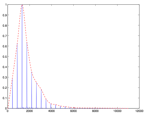
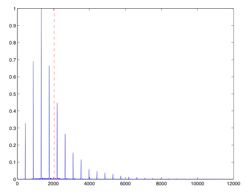
In figure 6.4, the dashed red line represents the spectral envelope, and simply connects the peaks of the spectrum. It should be noted that there is no one correct way to produce a spectral envelope, since it requires the determination of what constitutes a “peak”, which is a complicated and subjective task.

Spectral Centroid

The spectral centroid represents the center of mass of the spectrum, and is strongly correlated with our preception of the brightness of a sound. Generally, the higher the value of the spectral centroid, the brighter a sound will be judged to be.

The spectral centroid is a weighted average of the magnitudes a spectrum: \begin{equation} C=\frac{\sum_{n=0}^{N-1} f(n) a(n)}{\sum_{n=0}^{N-1} a(n)} \label{eq:spectralcentroid} \end{equation} where \(n\) is the sample number, \(N\) is the number of samples in the spectrum, \(f(n)\) and \(a(n)\) are the frequency and amplitude of bin \(n\), respectively.

The spectrum of a trumpet playing A4 (440 Hz) fortissimo. The red line shows the spectral centroid. Compare with the figure below to see how it moves when the same note is played quieter.

(Image by John MacCallum)

(Audio by John MacCallum)

The spectrum of a trumpet playing A4 (440 Hz) pianissimo. The red line shows the spectral centroid. Compare with the figure above to see how it moves when the same note is played louder.

(Image by John MacCallum)

(Audio by John MacCallum)

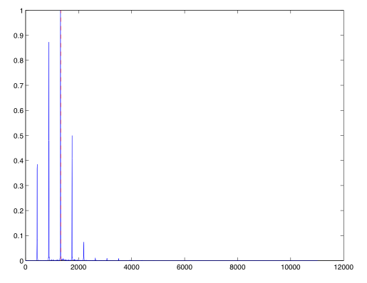
Figures 6.5 and 6.6 both show the spectrum of a trumpet playing A4 (440 Hz), the top fortissimo, and the bottom pianissimo. When played fortissimo, the spectral centroid is well above the peak with the largest magnitude; this is due to the contribution of the energy in the higher partials to the right of that peak. In the bottom plot, the energy falls off rapidly after the third partial, and we can see that the spectral centroid is noticeably lower. This should correlate with our experience of brass instruments which generally become brighter as they get louder.

Formants

Formants are concentrations of energy in particular areas of the spectrum. and are usually seen as broad peaks (local maxima) in the spectral envelope. They are particularly useful in the analysis of vocal timbre: the general distinction between different vowels and the characteristic timbre of different people’s voices, and those of men, women, and children, can be described in terms of their formant structure. In the voice, formants are the result of resonant structures in the vocal tract, while rooms can be said to have formants as well, due to their geometry construction, feature that was exploited to great effect by Alvin Lucier in his recording I Am Sitting in a Room.

The formant structure of three different vowel sounds.

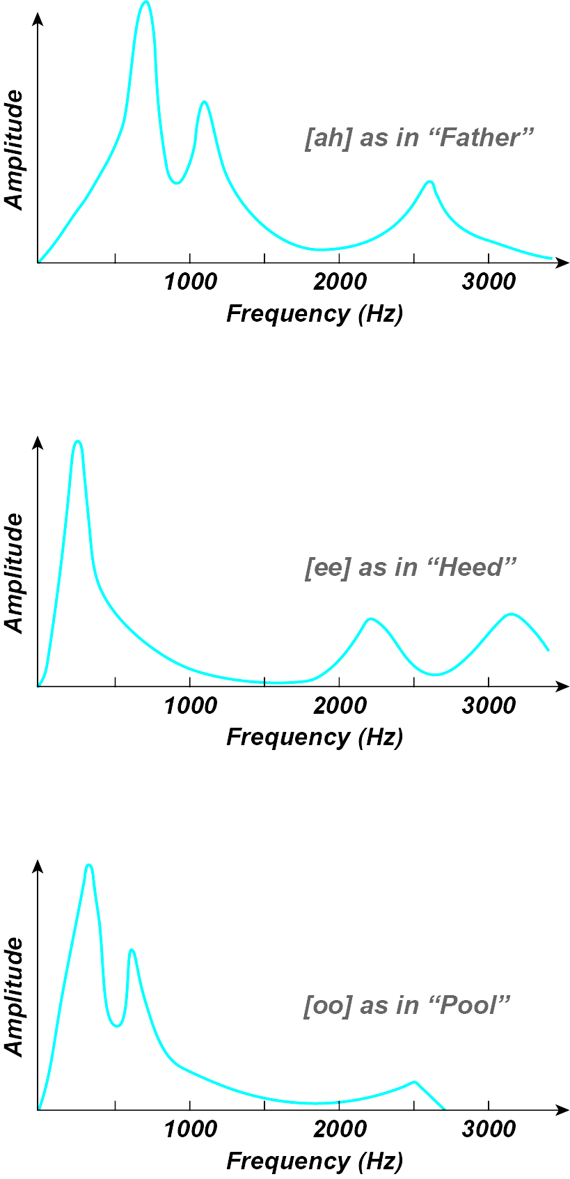
Figure 6.7 shows the formant structure of three different vowels. (Image by James Cheung. Adapted from Benade, 1976)

Average formant locations for men, women, and children across a number of different vowels.

	Formant	HEED	HEAD	HAD	HOD	HAW’D	WHO’D
Male	F1	270	530	660	730	570	300
Male	F2	2290	1840	1720	1090	840	870
Male	F3	3010	2480	2410	2440	2410	2240
Female	F1	310	610	860	850	590	370
Female	F2	2790	2330	2050	1220	920	950
Female	F3	3310	2990	2850	2810	2710	2670
Child	F1	370	690	1010	1030	680	430
Child	F2	3200	2610	2320	1370	1060	1170
Child	F3	3730	34570	3320	3170	3180	3260

Table 6.1 shows the average center frequencies for the first three formants of male, female, and child voices across a range of vowel sounds. Although we all have different voices, and our ability to distinguish the voices of people we know is remarkable, this table gives a reasonable estimate of the general position of these formants.

Local Features of the Spectrum that Relate to Timbre

In addition to the global features of the spectrum discussed above, our perception of timbre also depends, to some extent, on more local features, such as the balance of the strengths of certain partials with respect to others.

Even / Odd Balance

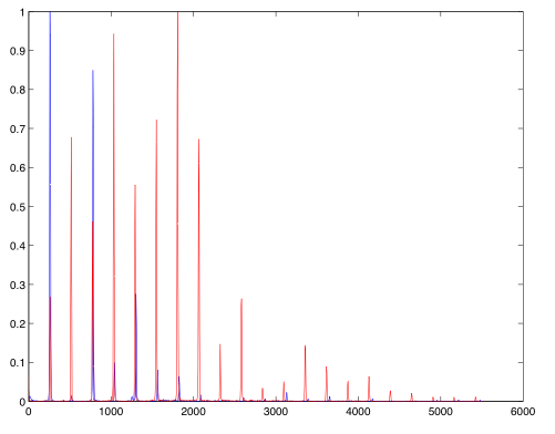
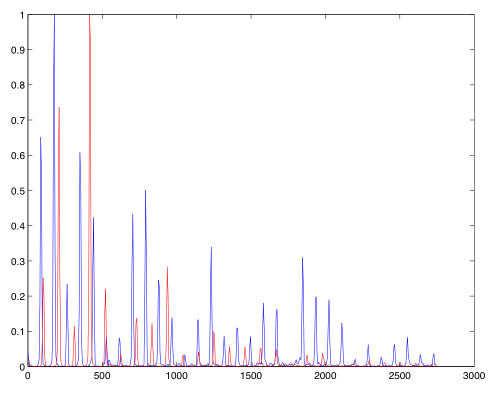
The relative balance of even to odd harmonics can have a profound impact on the timbre of a sound. Most notably, the middle and low registers of the clarinet have very weak even partials; compare the two plots of a cello (red) and a clarinet (blue) both playing (middle) C4 (261 Hz) inthe figure below.

The spectra of a cello (red) and a clarinet (blue) each playing C4 (middle C). Note that the even partials of the clarinet have almost no energy.

(Image by John MacCallum)

The missing even partials contribute to the “woody” or “hollow” sound characteristic of the clarinet.

Harmonicity

So far, we have only considered instruments that produce sounds that have their energy distributed along the harmonic series, i.e. the harmonics are all equal multiples of some fundamental. Many sounds, particularly those made by percussion instruments, do not behave this way—we refer to those timbres as inharmonic. The configuration of partials of inharmonic sounds can be hugely varied, and quite complex. They can often produce the sensations of roughness or sensory dissonance that we discussed in unit 4

.

Proximity of Partials to one Another

Another characteristic involves inharmonic components, usually part of the attack transient (more on that below), that are in close proximity to the components that give the sound its more recognizable quality. When this happens, the closely spaced partials beat against each other, producing the sensations of beating, sensory dissonance, or roughness that we discussed in unit 4

Sensory Consonance and Dissonance

Temporal Evolution of the Spectrum

As we mentioned at the beginning of this unit, sounds are continually changing, and the way a spectrum changes over time contributes a great deal to our perception of a timbre.

Temporal Envelope

The temporal evolution of many sounds, may be broken down into a sequence of distinct parts. Instrumental sounds, for example, often follow the familiar pattern:

attack: the initial onset of the sound—despite the name, this can be long and slow, or a short burst of energy,

(decay): a short decrease in energy following the initial onset (often omitted in descriptions of envelopes),

sustain: a relatively static portion of the sound where the spectrum is relatively stable,

release: the way in which the sound transitions to silence.

The temporal envelope of a sound, showing a common segmentation into four parts: Attack, Decay, Sustain, and Release (ADSR).

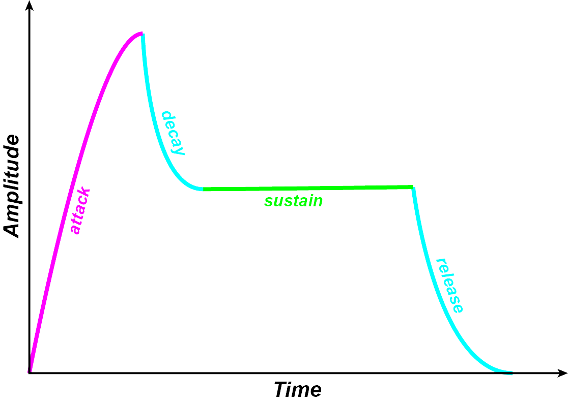
(Image by James Cheung)

As with timbre itself, these 3–4 stages of the temporal evolution of a sound are not intrinsic to any sound—they are subjective determinations made for the purposes of discussion, modelling, etc. That said, the first few milliseconds of a sound play an important role in the way we experience the subsequent parts of that sound.

In the following sequence of examples, the attack and release have both been removed. See if you can figure out which instrument produced them.

Attack and release removed	Original

(Audio files by John MacCallum)

Onset of Partials

As we just heard, the opening milliseconds of a sound communicate a great deal of information about it—this is why it is important that when we conceptualize timbre as related to the spectrum, we don’t stop there. The way in which the energy distribution changes over the course of those first few milliseconds can leave just as much of a stamp on the sound and our impression of it as the more steady-state parts, and likewise with the decay or release.

The attack of a Bb clarinet playing A4 (440 Hz) mezzo-forte. Note the staggered entry of the partials.

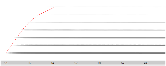
(Image by John MacCallum) In figure 6.10, we can see how the partials enter (the energy distribution changes) during the attack of a clarinet playing A4 mezzo-forte. Generally, we can say that the timbre gets brighter as the tone gets louder, and this can be seen in the figure as more and more energy becomes present in the upper part of the spectrum.

Transients

In addition to the changing distribution of energy we just saw, there is often noise associated with the attack of a sound. Technically, this also represents a gange in the distribution of energy, however, it can be differentiated from that of the entry of the partials we saw above. We refer to the frequency components of these bursts of energy as transients. They are typically very short, and caused, for example, by the initial noise of a reed begining to vibrate against the lips and mouthpiece, the initial burst that gets the lips buzzing in the mouthpiece of a brass instrument, the initial slipping of the string against the hair of a bow, etc.

A sonogram of a bell from the Sather Tower Campanile on the UC Berkeley campus. Note the noise burst that occurs when the bell is struck.

(Audio by John MacCallum)

In the example above, the transients can be heard and seen as a momentary burst of inharmonicity in the opening milliseconds of the sound.

Timbre and Orchestration

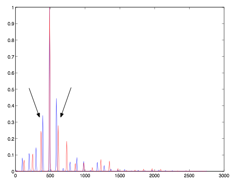
In orchestration, the blending of timbres is a primary concern. There is no one right or good way to orchestrate or blend timbres together—this is dependent on intention. However, we can easily show what we already know from experience: one pair of instruments playing a dyad can produce quite a different result than another playing the same dyad. For example, compare the spectra of two cellos playing a low major 3rd (Gb-Bb), with that of two bassoons playing the same interval.

Spectra of two cellos playing G2 and B2.

(Image by John MacCallum)

Spectra of twy bassoons playing G2 and B2, the same interval as above. Note the tightly spaced partials pointed to by the arrows.

(Image by John MacCallum)

In figure 6.13, the peaks that surround the one at 500 Hz are strong, and slightly mistuned, resulting in a perceptually dissonant version of what should be a functionally consonant interval. In figure 6.12, there is still an aspect of dissonance, but it will not be nearly as strong.

Klangfarbenmelodie

The type of timbral variation on the same pitches we saw above was explored in a melodic fashion by Arnold Schoenberg in the third of his Fünf Orchesterstücke, Op. 16, which opens by alternating between two different orchestrations of the same chord:

The two orchestrations of the opening chord of Schoenberg's Farben.

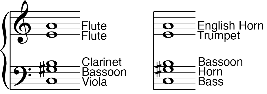
(Image by James Cheung. Adapted from John MacCallum)

The title of this short piece, Farben is German for color, and the term Klangfarben, or tone color can be translated as timbre. Schoenberg referred to this opening as a Klangfarbenmelodie, or tone color melody. Schoenberg chose this alternation to explore whether timbral contrasts could replace tonal tension in atonal music, i.e. music that is not characterized by a dominant-tonic relationship.

Building on the discussion in the beginning of this section, MacCallum and Einbond showed (MacCallum et al., 2008) that the choice of these two orchestrations are significantly different from each other, and from a “pure” sine-tone rendering.

With pure tones, the notes of the chord are generally well outside the critical band from one another, and as we saw in unit 04 , will not produce much sensation of roughness. The two orchestrations, however, are quite rough, due to the orchestration chosen.

An analysis of the spectra of the two orchestrations of the 'Farben' chord, in comparison with a rendering of pure sinusoids.

(Image by John MacCallum)

Timbre Space as a Musical Control Structure

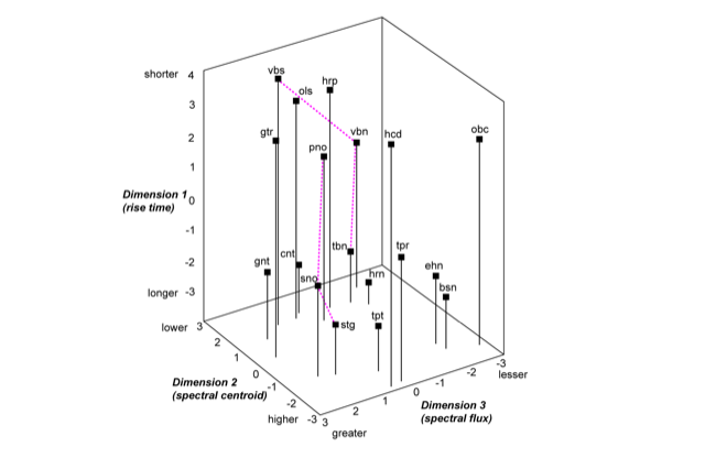
Despite the importance and complexity of timbre, it is often seen as less important musically than rhythm, harmony, melody, etc. In 1978, David Wessel wrote a paper called “Timbre Space as a Musical Control Structure” (Wessel, 1979), that, as he described, was in response to a disagreement between himself and Pierre Boulez about the ability for timbre to play a structural role in music. Wessel also makes references to the 1975 paper “An exploration of musical timbre” in which John M. Grey describes how he applied the multi-dimensional scaling method to data obtained from similarity ratings of the timbres of musical instruments. Based on these ratings, he was able to derive two- and three-dimensional representations of timbre space characterized by the dimensions attack time, centroid and spectral flux (a measure of how energy moves from lower to higher partials over time)

Two-dimensional timbre space representation of 24 instrument-like sounds obtained from Grey and quoted by David Wessel. Abbreviations for stimulus points : O1, O2 = oboes, FH = French horn, BN = bassoon, C1 = E-flat clarinet, C2 = bass clarinet, FL = flute, X1 X2, X3 = saxophones, TP = trumpet, EH = English horn, S1 = cello played sul ponticello, S2 = cello played normally, S3 = cello played muted sul tasto, FHZ = modified FH with spectral envelope, BNZ = modified BN with FH spectral envelope, S1Z = modified S1 with S2 spectral envelope, S2Z = modified S2 with S1 spectral envelope, TMZ = modified TM with TP spectral envelope, BCZ = modified C2 with 01 spectral envelope, 01Z modified 01 with C2 spectral envelope.

(Image by Janina Luckow. Adapted from (Wessel, 1979))

In the three-dimensional representation, the dashed lines, suggest that timbre space can be used as a control structure in which timbre modulations and transpositions can be achieved in analogy to the pitch and key spaces.

Three-dimensional timbre space representation of sounds obtained from single instruments and hybrids (several instruments playing together). Abbreviations: bsn=bassoon, cnt = clarinet, ehn = English horn, gnt = guitarnet (guitar+clarinet), gtr = guitar, hcd = harpsichord, hrn = French horn, hrp = harp, obc = obochord (oboe+harpsichord), ols = oboleste (oboe+celeste), pno = piano, sno = striano (bowed string+piano), stg = bowed string, tbn = trombone, tpr = trumpar (trumpet+guitar), tpt = trumpet, vbn = vibrone (vibraphone+trombone), vbs = vibraphone

(Image by Janina Luckow. Adapted from (Wessel, 1979))

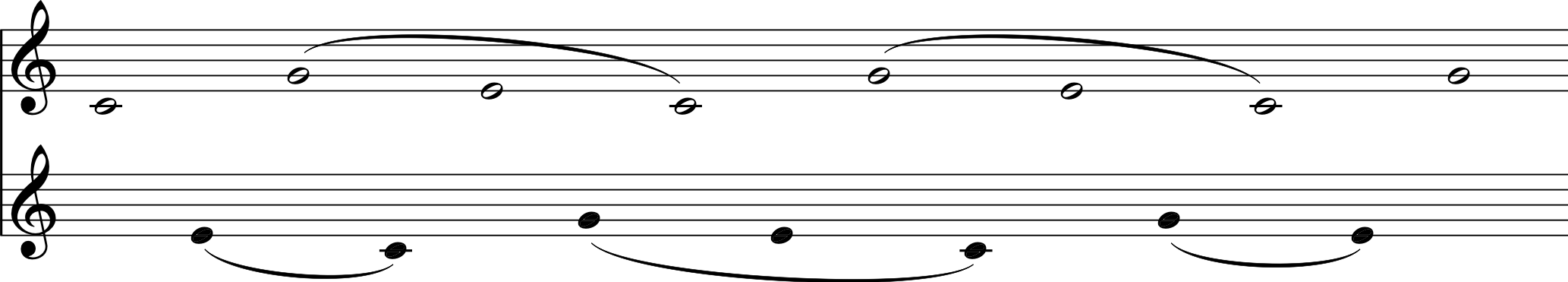
In order to demonstrate the ability of timbre to override other musical structures by “stream segregation”, he devised what would later become known as the “Wessel Illusion”: a simple ascending major is played repeatedly by two different timbres that alternate notes, as shown in the figure below.

Wessel Illusion: the black noteheads represent one timbre, and the white, another.

(Image by James Cheung. Adapted from (Wessel, 1979))

As the tempo increases, gradually the two timbres “split apart” into their own descending melodies, as shown below.

Wessel Illusion: as the tempo increases, the percept switches from a single repeated ascending line, to two descinding lines.

(Image by James Cheung. Adapted from (Wessel, 1979))

Max Example: David Wessel's Illusion

(Max Patch by Víctor Gutiérrez John MacCallum and Georg Hajdu)

you can have access to all MUTOR interactive Max patches when you download the maxpatches folder inside the MUTOR github repository and include it in the Max search path.

Quiz

1. Define timbre.

2. What measurement does our perception of sonic “brightness” correlate to? How?

3. What are formants? How do they contribute to speech?

4. Describe the difference between the “temporal envelope” and the “spectral envelope”.

References

1. Wallmark, Z. “Describing sound: The cognitive linguistics of timbre”. In ‘Oxford Handbook of Timbre, Oxford University Press’. 2018. 10.1093/oxfordhb/9780190637224.013.14
2. MacCallum, J. & Einbond, A. “Real-Time Analysis of Sensory Dissonance”. Computer Music Modelling and Retrieval, R. Kronland-Martinet, S. Ystad, and K. Jensen (Eds.), LNCS 4969, pp. 203-211. Springer-Verlag, Berlin, Heidelberg. 2008.
3. Wessel, D.L. “Timbre space as a musical control structure”. Computer Music Journal, 3(2): 45-52. 1979.
4. Grey, J.M. “An exploration of musical timbre”. Stanford University. 1975.

Authors

• John MacCallum and Georg Hajdu

Topics

• timbre
• spectrum
• spectral envelope
• temporal envelope
• attack

Contents