Unit 4: Consonance and Dissonance
Synopsis
What makes some sounds dissonant? Is dissonance a property of sounds themselves, or is it part of our perception of sound? Throughout history many attempts have been made to model dissonance. Early models dating back 2500 years to Ancient Greece and China were geometric in nature, that is, they considered musical intervals as ratios of two string lengths and showed that certain kinds of ratios were associated with consonant intervals, and others with dissonant ones. Today, our models of consonance and dissonance also take into account our understanding of the anatomy and functioning of the inner ear, particularly the basilar membrane, as well as the ways in which temporal fluctuations associated with the perception of dissonance are encoded and transmitted along the auditory nerve and in the Inferior Colliculus. Further, we are able to say that certain high-level cognitive processes can override lower-level sensation, producing judgements of consonance or dissonance that can contradict both physical and anatomical sensation. Taken together, these different perspectives comprise our current models of consonance and dissonance.
- What do we mean by “Consonance” and “Dissonance”?
- Early Models of Consonance and Dissonance
- Context Matters
- Tonotopic Organization of the Ear
- Critical Bands, the Basilar Membrane, and Frequency Selectivity
- Bandwidth and Shape of the Auditory Filter
- “Roughness” and Discrimination
- Complex Tones
- Sonorities of More than Two Tones
- Top-Down Processing and Its Effect on Dissonance
- Neurobiology of Consonance and Dissonance
- Quiz
- References
What do we mean by “Consonance” and “Dissonance”?
The terms “consonance” and “dissonance” are antonyms of one another, the former meaning “sounding together”, while the latter means “not sounding together” or “a lack of consonance.” This circular definition of dissonance makes it difficult to understand what dissonance is on its own terms, outside of its relational context with consonance. The New Grove Dictionary of Music and Musicians defines dissonance as “a discordant sounding together of two or more notes perceived as having ‘roughness’ or ‘tonal tension.’” This definition points to properties that dissonance has, rather than what it lacks, however, the definition requires the reader to understand what “roughness” and “tonal tension” might mean, two quite technical terms. But even in this short definition, we can see that the term “dissonance” is associated with two different concepts: one perceptual, alluded to by the term “roughness”, which we will discuss later in this unit, and one contextual, as “tonal tension” requires exposure to, and some degree of education in European tonal music. These two ways of considering dissonance correspond roughly to cognitive processing from the “bottom-up” and “top-down”, concepts that we will continue to encounter throughout these units.
Early Models of Consonance and Dissonance
We can say for sure that these terms imply the presence of more than one sounding object in order to be judged as “sounding together” or “not sounding together.” It would seem then that consonance and dissonance might be situated in the relationship of multiple objects sounding simultaneously, and indeed, this is what Pythagorus proposed.
He observed that two strings of different lengths vibrating simultaneously produced consonant intervals when the ratios of the string lengths consisted of small whole numbers, and dissonant intervals otherwise. For example, when the string lengths are in a ratio of 1:1, that means that they are the same length, and sound together as one, or in “unison.” When one string is twice the length of the other, a ratio of 2:1 produces an “octave”, while ratios 3:2 and 4:3 produce a “fifth” and a “fourth” respectively. Multiples of these ratios, such as 4:1, 3:1, 6:2, 8:3, etc. simply add an octave to the interval. Ratios of larger numbers that cannot be further reduced, such as 9:8, a major second, are dissonant.
For Pythagorus, the intervals of the octave (2:1), fifth (3:2), and fourth (4:3) are all equally consonant, however, there is a problem. Let’s say we tune two strings $s_1$ and $s_2$ to the ratio of a fifth, 3:2, that is, $s_1$ is 1.5 times longer than $s_2$. Now let’s add a third string, $s_3$, in a 3:2 relationship with $s_2$ (again, $s_2$ is 1.5 times longer than $s_3$). The ratio between $s_1$ and $s_3$ is now 9:4, or a major second plus an octave. If we continue this process for a total of 12 steps, we arrive at a ratio that is very nearly, but not exactly, 7 octaves above the pitch that we started from, since the ratio of 3:2 applied 12 times, $1.5^{12} = 531441$ is not the same as the ratio of 2:1 applied 7 times, $2^7 = 524288$. This descrepancy, itself expressed as a ratio, $1.5^{12} / 2^4 = 531441 / 524288 \approx 1.01365$, is often referred to as the Pythagorean comma. The existence of the comma can be interpreted as follows: perfect fifths and octaves cannot both be perfectly in tune at the same time, but rather, some sacrifices in intonation must be made in order to distribute this error among the different intervals. There is not a single right answer to the question of how to do this; the decision must be made in a musical context with particular repertoire in mind, and for this reason, there are hundreds of intonation strategies, of which equal temperament is currently the most pervasive.
The set of observations made by Pythagorus and Chinese mathematicians in the same era, that it is possible to determine whether an interval is consonant or dissonant mathematically, could be considered one of the earliest attempts to model the phenomenon of consonance and dissonance. Importantly, it constructs consonance and dissonance as objective properties of sounding objects, but does little to explain what it is about these ratios that would make them sound the way they do.
Context Matters
The discussion of intonation and the Pythagorean comma above is our first clue that modeling consonance and dissonance may not be so simple. If you cannot have both fifths (and by inversion, fourths) and octaves in tune at the same time, we have to ask how far out of tune an interval can be before it transitions from consonant to dissonant, and similarly, when does an interval that is very close to 3:2, but not exactly 3:2 stop sounding like a fifth?
The next clue can be found by looking at the treatment of the fourth, which historically has been considered both a dissonant and a consonant interval . For example, in common practice tonal music, a fourth that appears as the lowest interval of a harmony is considered a dissonance and must be prepared and resolved properly, while a fourth that appears between the inner or upper voices is considered consonant and needs no special treatment.
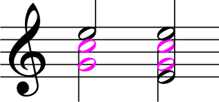
(Image by James Cheung)
|
| |
|
| |
(Audio by Víctor Gutiérrez)
This suggests that context matters, and the attribution of “dissonant” or “consonant” to an interval, the physical, sounding object, may not tell the whole story. Importantly, the judgement that a fourth on the bottom of a sonority is dissonant, while in other places it is not, is not simply a matter of style, or an arbitrary rule we learn in our music theory class. We actually perceive the fourth differently when it is in these different configurations, and to understand the reason why, we will need to consider the notes that make up intervals as complex tones with spectra, as well as to look at our physiology and the way we perceive frequency.
Tonotopic Organization of the Ear
In the 19th century, German physicist and physician Hermann von Helmholtz formulated Ohm’s acoustic law which states that the human ear perceives musical sound by decomposing it in a manner similar to the Fourier transform. Building on the idea that the ear decomposes complex sounds into a sum of simple ones, he went on to explain the relationship between musical consonance and simple frequency ratios on the basis of the appearance of “beats” that occur when two tones have a very small difference in frequency. As noted some 100 years later by Plomp and Levelt (Plomp et al., 1965), this idea is not without controversy and has been “severely critiqued” from a number of angles. Nevertheless, the notion that the ear is somehow sensitive to the different frequencies present in a complex tone was demonstrated by Hungarian biophysicist Georg von Békésy in the 1930s. Using state of the art stroboscopic photography, he was able to show that the basilar membrane vibrates like a surface wave when stimulated by a tone, and that due to the conical shape of the cochlea in which it resides, the location of the maximum peak of this wave varies according to frequency, meaning that this organ is tonotopically organized, as we saw in unit 2. Put another way, the continuum of (audible) frequency is mapped from low to high from one end of the basilar membrane to the other.
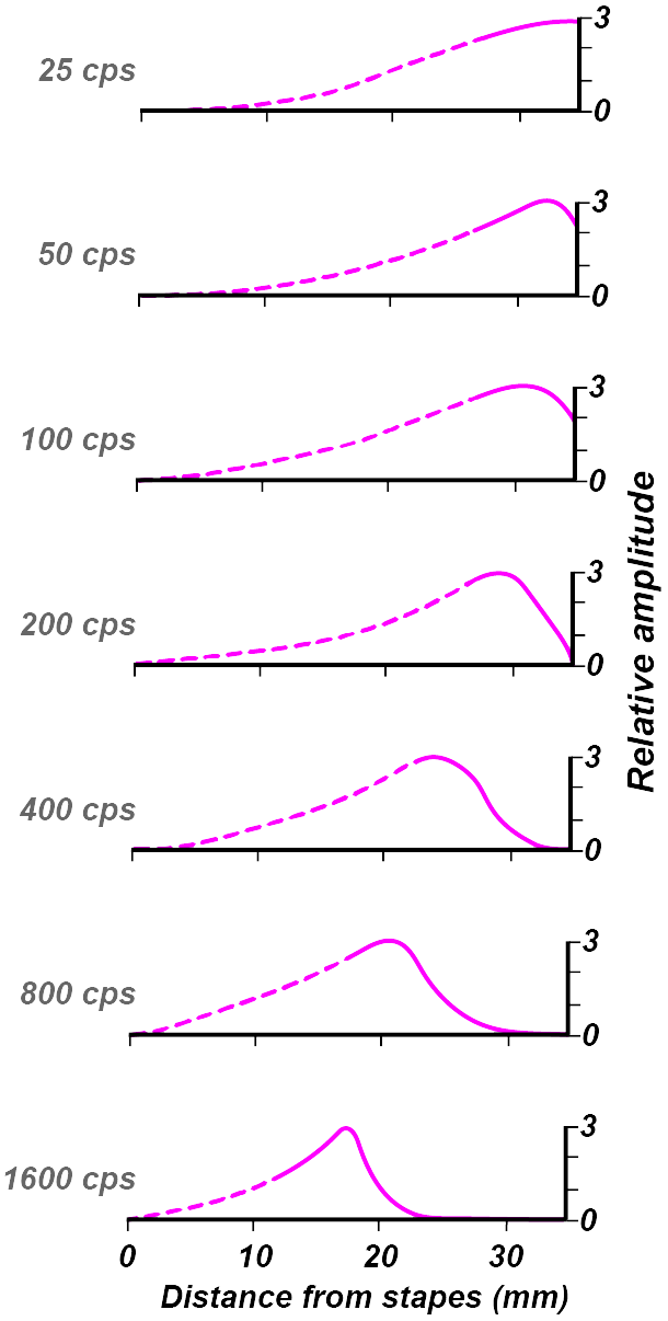
(Image by James Cheung. Adapted from (von Békésy, 1961)) Figure 4.2 shows von Békésy’s measurements of the displacement of the basilar membrane in response to auditory stimuli of different frequencies (von Békésy, 1961).
Critical Bands, the Basilar Membrane, and Frequency Selectivity
Around the same time that von Békésy was working in the 1930s, US physicist Harvey Fletcher introduced the notion of the “critical band”, which describes the behavior of the cochlea in terms of a series of overlapping filters (Fletcher, 1940). In the 1960s, Plomp and Levelt showed that “the transition range between consonant and dissonant intervals is related to critical bandwidth” (Plomp et al., 1965).
Simple-tone intervals are evaluated as consonant for frequency differences exceeding this bandwith, whereas the most dissonant intervals correspond with frequency differences of about a quarter of this bandwidth. (Plomp et al., 1965)
They go on further to discuss issues related to that of the perfect fourth described above, namely that given two notes sounding simultaneously, the overall quality of consonance or dissonance is related to the relationship of the overtones to one another with respect to the critical band. Put another way, certain intervals may sound more or less dissonant depending on what instruments are playing them, and what other notes are sounding simultaneously.
Bandwidth and Shape of the Auditory Filter
The frequency resolution of the auditory filter is directly related to the frequency selectivity of the hair cells along the basilar membrane. Extensive psychoacoustical experiments have been conducted in order to measure the bandwidth of the auditory filter, or critical bandwidth. Based on these measurements, we are able to build a model of the filter and observe its response to different sounds. Around middle C (approximately 250Hz) the critical bandwidth of the auditory filter is about 1/3 of an octave wide. (We can, however, differentiate pitch at much higher resolutions – we will discuss why later.) In lower registers (bass frequencies) the critical bandwidth is wider, spanning up to an octave. Hi-fi audio systems generally use 1/3 octave bands which provide a fairly good match to the resolution of the auditory filter.
Many formulae have been constructed to estimate the width of the critical band as it varies with frequencies. The most accurate of these formulae is the Equivalent Rectangular Bandwidth (ERB), which is given by \begin{equation} \mathrm{ERB}(f) = 0.108f + 24.7 \label{eq:erb} \end{equation} Using this formula, we can simulate the basilar membrane using a bank of gammatone filters. with a frequency response described by \begin{equation} \gamma(t) = at^{n-1} e^{-2\pi bt \mathrm{ERB}(f_c)} \mathrm{cos}(2\pi f_c t + \phi) \label{eq:basilar_membrane_fb} \end{equation}
(Image by John MacCallum)
“Roughness” and Discrimination
The picture that is beginning to emerge is that consonance and dissonance are not binary opposites of one another. Rather, as two tones approach each other in frequency, as they enter the critical band, our perception of them shifts, and we begin to experience them as a single percept with a frequency roughly equal to the average of the two that has a “rough” quality to it.
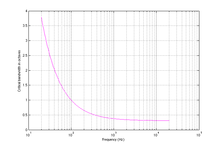
As the $\mathrm{ERB}$ formula indicates, the size of the critical band varies with frequency, and can be quite large in the low register. The following two figures plot the width of the critical band as a function of frequency, first in hertz, and then in octaves.
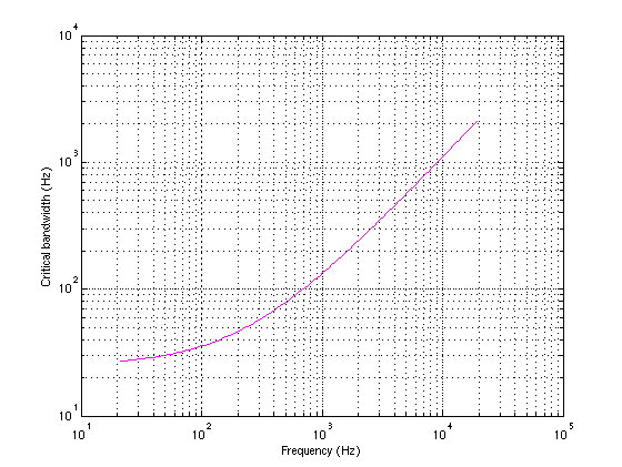
(Image by Janina Luckow)
(Image by Janina Luckow)
As we can see, at a frequency of 200 Hz, the critical band is an octave wide, indicating that even when two tones are separated by a large musical interval, we have a difficult time hearing them as seperate phenomena when they are in the bass register. This also confirms what many musicians already know, which is that intervals that are normally considered consonant like thirds, can sound rough and dissonant (muddy) in the low register.
(Max Patch by Víctor Gutiérrez and John MacCallum)
you can have access to all MUTOR interacive maxpatches when you download the MUTOR github repository inside the maxpatches folder.
Complex Tones
The roughness or smoothness of a complex sonority is dependent to some degree on the number and configuration of the partials associated with each component of the sound. Two pure tones whose frequencies reside outside a critical band will be perceived as relatively smooth, however, depending on the interval between them, as the number and strength of their partials increases, the sonority may increase in roughness if upper partials fall within critical bands. For example, when composed of pure tones, a major 7th built on the C above middle C is quite smooth as the two frequencies are well outside the critical band. If overtones are added, however, the first overtone of the lower note will be a minor second away from the fundamental of the top note, not only well within the critical band, but within the lower 1/4th of the critical band, which Plomp and Levelt describe as being the area correlated with the strongest sense of dissonance.
Interestingly, experiments have shown that non-musicians tend to rate a major 7th as smooth when it is made up of pure tones, while musicians rate it as dissonant, suggesting that our pre-existing knowledge and expectations of music, or top-down understanding, play a role in the perception of roughness, and giving us another clue that answers to questions of consonance and dissonance are not necessarily located in the sounding objects.
Sonorities of More than Two Tones
Up to now, we have been been concerned primarily with dissonance as it relates to diads, but what about more complex sonorities containing many pitches? Often, a reasonable estimate of the overall roughness of a sonority can be found by simply summing the roughness contained in each band of the auditory filter.
Using a formula for estimating the roughness of a sonority designed by Richard Parncutt and modified by (MacCallum et al., 2008), we can assign roughness values to three different orchestrations of the opening chord from Arnold Schoenberg’s work Farben, Op. 16.
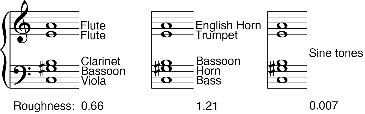
(Image by James Cheung)
|
| |
|
| |
|
| |
As can be seen in figure 4.7, and heard in the audio examples, the sonority is quite smooth when played with pure tones, however, the two different orchestrations provided by Schoenberg are relatively rough in comparison, and very different from each other. This can partly be explained by looking at the spectra in the figure below.
(Image by John MacCallum)
In the second of Schoenberg’s orchestrations, the rougher of the two, we can see that there is a strong partial at a frequency of 495.3 Hz, that is not present in the first orchestration, that is well within the critical band of the neighboring component at 522.2 Hz. 495.3 Hz corresponds to the B above middle C and is the second partial above the B played by the clarinet in the first orchestration, and the bassoon in the second. A missing second partial is a known characteristic of clarinets, and contributes to their “hollow” sound, and has been used to great effect by composers, as in this example, long before the phenomena described in this unit have been well understood from a scientific perspective.
In some cases, however, simply adding the roughness of each filter together to estimate the overall roughness of a sonority will not provide a good model. An example can be found in the opening sonority of György Ligeti’s Atmosphères, which is a massive cluster of semitones spanning a large part of the orchestral range.
|
| |
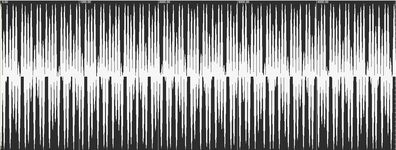
If our simple additive model of roughness held, this should be an extremely dissonant chord, where in fact the experience of it is as quite a smooth sonority. This is likely due to the effects of phase cancellation which result in a waveform with minimal amplitude modulation. A simple example of this can be seen here:
(Image by John MacCallum)
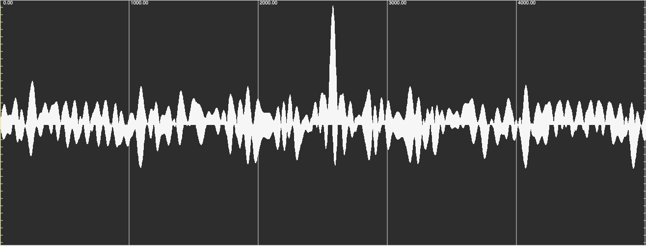
(Image by John MacCallum)
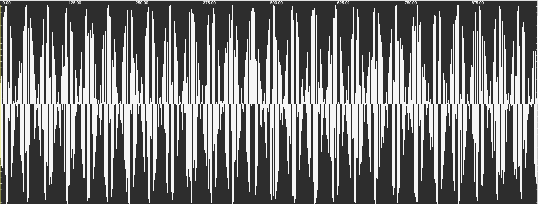
(Image by John MacCallum)
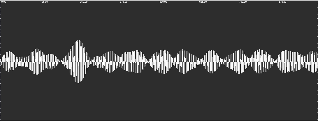
(Image by John MacCallum)
|
| |
|
| |
Figure 4.12 presents two waveforms, one containing a sum of two sinusoids a minor second apart, and the next containing 40 sinusoids summed together inside that same interval. As we can see in the bottom two closeup images, the extent of the amplitude modulation in the bottom plot is greatly reduced than that of the minor second.
Top-Down Processing and Its Effect on Dissonance
Counterpoint and the Wright-Bregman Hypothesis
As sounds become increasingly separated into different streams (where streams can refer to spatial location in this case), beating diminishes and sound less rough. This explains why binaural beats do not sound as rough as monaural beats. Wright and Bregman
propose that certain auditory cues such as stream segregation can prevent the listener from hearing dissonant intervals as such. The figure below is an example taken from Auditory Scene Analysis ; in the top example, although the boxed intervals are dissonant, that dissonance is supressed by the strong separation of the two lines into separate streams. In the bottom example, the streaming cues are not present and the same intervals are heard as dissonant.
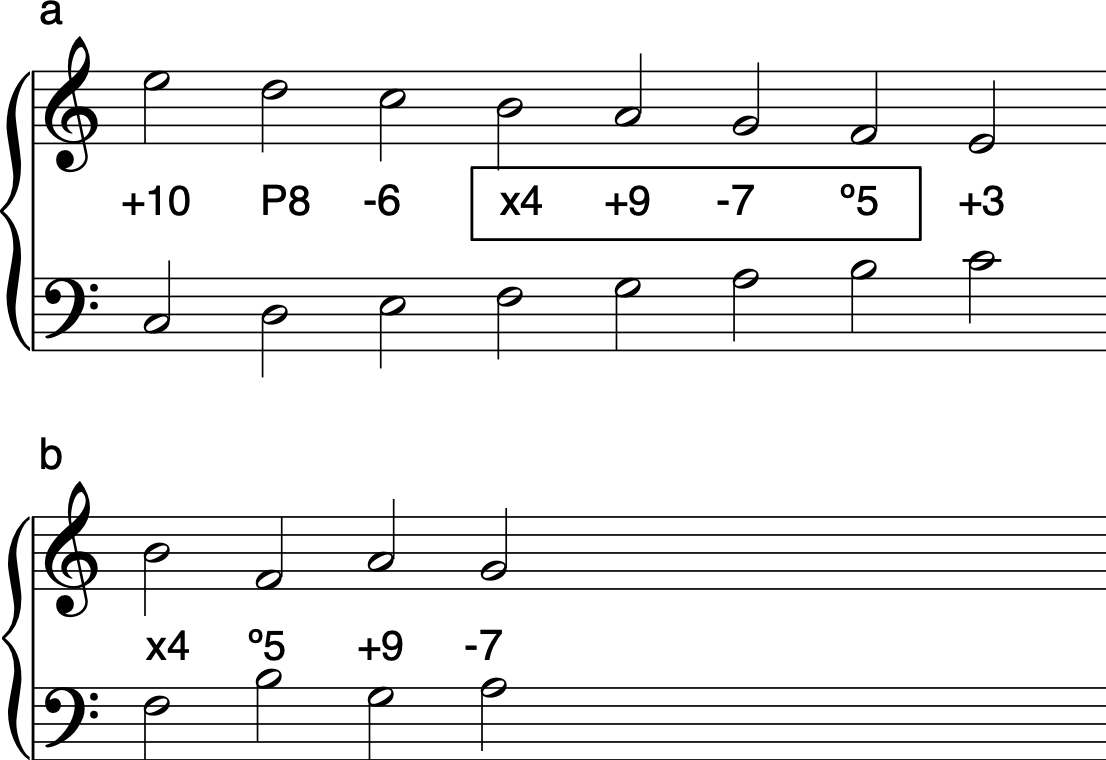
(Image by James Cheung)
The separation of sounds into streams is heavily influenced by top-down processes such as attention and long-term memory. Thus top-down influences on perception of consonance and dissonance begins to be important at this level. Referring back to Terhardt’s two-component theory , factors contributing to musical consonance (as opposed to sensory consonance) include spatial localization, musical texture, and stream segregation, all of which are sensitive to top-down modulations.
David Huron has proposed that stream segregation and related perceptual principles give rise to our existing rules of counterpoint and voice-leading. Traditional voice-leading practices in this view include: the use of three to four distinct voices, the prominence of stepwise motion rather than leaps in each voice, and the avoidance of parallel fifths and octaves. These compositional practices may result from the perceptual principles of auditory streaming and source segregation. In order for each individual voice to be perceived as one stream, the perceptual principle of pitch proximity dictates the use of stepwise motion. Additionally, for distinct voices to be perceived as separable streams, frequency and amplitude comodulation are generally avoided, giving rise to the avoidance of parallel motion. These are only some of the ways in which compositional practices are governed by perceptual principles.
Other Factors Contributing to Roughness
In addition to the interaction of two tones within close frequencies, some other factors that contribute to our perception of roughness include spatial location, phase-related fluctuations, and mistuning of consonant intervals.
Spatial location: is important because it is a cue for the auditory system to compute the difference between input to the two ears. Although beats can arise monaurally from sounds mixing before they enter the ear, they can also arise neurally when sounds come together within the binaural system. The interaction of sounds presented binaurally results in binaural beating.
Phase-related: fluctuation occurs when partials in a harmonic complex are not phase-locked. When the carriers of two amplitude-modulated tones are modulated in phase, the summated roughness is about twice that of either of the amplitude-modulated tones alone. Summated roughness is least when the modulations are anti-phase. Phase-locking is necessary for this to occur.
Beating of mistuned consonances: is another phenomenon related to the perception of roughness and beating. It is a reported phenomenon that beating is perceived when two simultaneously tones are played at frequencies that deviate very slightly from small-integer ratios. For example, a slightly mistuned octave will beat at the frequency at which the higher tone deviates from twice the lower tone; i.e. a 500Hz tone and a 1005Hz tone will beat at 5Hz . The origin of this phenomenon is unknown, but it is shown to be largely dependent upon the level and frequency of the lower component. Viemeister et al (2001) suggest that the perception of beating of mistuned consonances seems to be more dependent upon the fluctuations of the amplitude envelope of the two tones, rather than the fine temporal structure, or information within the amplitude envelope.
Neurobiology of Consonance and Dissonance
In order to further understand the different types of top-down modulation on consonance perception, it is important to understand the auditory pathway and the processes acting on the neural representations of sound. Such a detailed anatomical pathway is laid out in another unit, but the present discussion will focus on the stages of the auditory pathway specifically related to consonance and dissonance perception.
Neural coding of dissonance seems to begin at the level of the auditory nerve. Tramo et al. (2001) report that the temporal fluctuations of the auditory nerve firing pattern are inversely correlated with consonance perception. Thus it seems that the auditory nerve is passing on dissonance-related information towards further levels of the auditory system.
The Inferior Colliculus (IC) is a structure in the midbrain that plays an important role in dissonance perception. In studies involving single-unit recordings in the anesthetized cat, have shown that neural firings of the IC correlate positively with amplitude modulation at the beat frequencies resulting from the interaction of two tones. Firings at the beat frequency were observed in the IC in response to simultaneously-presented minor 2nd tones for both pure and complex tones. IC firings also correlated with complex tones presented at a tritone apart (see the figure below). These findings suggest that the biological basis of dissonance between complex tones is coded at the midbrain level.
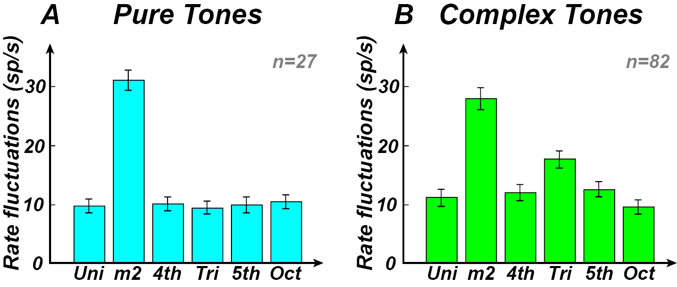
(Image by James Cheung. Adapted from Tramo et al. (2001))
Studies with lesion patients have also shown effects of consonance and dissonance at the level of the auditory cortex. Tramo et al. (2001) tested patients with bilateral A1 lesions and found that pitch perception and consonance perception were both impaired, but dissonance perception was intact. This led to their suggestion that consonance is an emergent property of the relationship between pitches of simultaneously-perceived tones, whereas dissonance is a function of roughness and beating which is independent of consonance.
Quiz
Define the auditory filter. What is the relationship between critical band and the Gammatone filter?
Which of the following sounds most dissonant?
- C4 and B4 played on pure tones
- C4 and B4 played on two clarinets on the opposite sides of a stage
- C4 and B4 played on two trumpets on the same side of a stage
- C4 and E4 played on two clarinets on the same side of a stage
Under what conditions are binaural beats most likely to be perceived?
Calculate the beat frequency of the second partials $(F_2)$ of complex tones with fundamentals at 440Hz and 441Hz respectively.
How does the Inferior Colliculus differentially encode pure tones and complex tones presented at a tritone apart?
According to the Wright-Bregman hypothesis, what factors may influence the perception of dissonance?
References
- von Békésy, G. “Concerning the pleasures of observing, and the mechanics of the inner ear”. Nobel Lecture. 1961.
- Plomp, R. & Levelt, W. J. M. “Tonal Consonance and Critical Bandwidth”. The Journal of the Acoustical Society of America 38, 548. 1965. 10.1121/1.1909741
- Fletcher, H. “Auditory Patterns”. Rev. Mod. Phys. 12, 47. 1940. 10.1103/RevModPhys.12.47
- MacCallum, J. & Einbond, A. “Real-Time Analysis of Sensory Dissonance”. Computer Music Modelling and Retrieval, R. Kronland-Martinet, S. Ystad, and K. Jensen (Eds.), LNCS 4969, pp. 203-211. Springer-Verlag, Berlin, Heidelberg. 2008.
Authors
Topics
- Consonance
- Dissonance
- Sensory Dissonance
- Critical Bandwidth
- Cochlea
- Basilar Membrane
- Timbre
- Intervals
- Tonotopic Mapping