Unit 1: The Auditory Stimulus
Synopsis
Our bodies contain complex organs that are sensitive to rapid variations in the air pressure around us. These pressure variations, along with different representations of them, are what we might call the auditory stimulus, that is the source of stimulation for the auditory sensors our bodies are equipped with. The auditory stimulus is the aspect of the complex phenomenon of sound that we all share, whether we hear it or not. It is the physical component of sound that travels from sources to receivers. The thing can be captured with microphones, recorded using analog and digital technologies, and played back with amplifiers and speakers. It is the thing represented when we read and write music notation. The nature of the auditory stimulus as fluctuations in the pressure of a medium over time means that it is not able to be directly captured; that is to say, the study of the auditory stimulus is really the study of the persistent physical traces it leaves behind as it interacts with objects sensitive enough to be displaced by it.
What Do We Hear?
Sound is all around us, invisible, yet ever present in our daily lives, but what exactly is it that we hear? In this unit, we focus on the physical phenomena that affect our perception of sound, and different ways we represent those phenomena.
When I make a sound, say I clap my hands together, I’ve produced a disturbance in the air that eventually travels to your ears, resulting in an effect that we ultimately describe as sound. This disturbance travels in every direction, reflecting differently off of every surface, the walls, the floor, the ceiling, bodies, furniture, etc. depending on their materials. This is all caused by air molecules bumping into each other; as they move away from the source of the sound, they create a region of higher pressure by compressing the space between themselves and their neighbors in the direction they are traveling. At the same time, the area in the opposite direction becomes a region of lower pressure, or a rarefaction. Our ears are particularly sensitive to these very fast and very small changes in pressure—you can think of our ears as extremely sensitive barometers.
When those changes in air pressure propagate into our ears, they transfer their energy through a complex array of anatomy, ultimately resulting in electrical impulses that travel up the nerve fibers from our inner ear to our brain, where we cognitively process this information as “sound”. The transfers of energy from one medium to another is called transduction, and the different parts of our anatomy through which these pressure waves are transduced as they make their way to our brain will be discussed in unit 2. For now, we will focus in this unit on the physical characteristics of sound waves, and the ways we represent them.
Recording and Representing Sound
|
| |
The image in figure 1.1 may be a familiar one—we might say we see a sound there, but it would be more accurate to refer to it as a waveform, as sound is something we perceive in time, rather than something we have and see as in this image. In order to produce a visual representation of something that sounds, we usually transduce the sound mechanically, such that its movements produce a visible trace on some medium. In the earliest recording devices, such as Thomas Edison’s phonograph cylinders, a needle, moved by sound vibrations, traced grooves in a wax cylinder. By reversing the process, i.e. spinning the cylinder while touching the needle to it and transferring the movement of the needle to a diaphragm, causing the tiny movements of the needle to displace a larger amount of air, the recorded sound could be played back, as shown in the video below:
The playback in such a device relies on analog amplification: a heavy, but small needle modulates a thin and light, but larger membrane that displaces a larger volume of air. Other recording and playback technologies involve the transduction of air movement into an electrical signal. This is done by using a small, light diaphragm to displace a coiled wire surrounded by a magnet. These small movements of the coil relative to the magnet alter the magnetic field and produce a very small electrical current, the voltage of which varies proportionally to the compressions and rarefactions of the sound.
Speakers work in the opposite way: an electrical signal is sent to a coil surrounded by a magnet, and the modulations in voltage displace the coil and a membrane, or speaker cone, attached to it, which moves the air back and forth.
Digital recordings make use of the analog electrical signal described above, but record the value of the voltage periodically, by sampling it, commonly at 44100 times per second. This is done using an Analog to Digital Converter or ADC, and the process is reversed by a Digital to Analog Converter or DAC, which modulates the voltage of an electrical signal proportional to the sampled values.
Analog and digital representations of sound are similar, but have some important differences. Perhaps most importantly, analog signals are continuous, while digital signals are discrete, i.e. they can be thought of as consisting of individual values that were recorded by taking samples of an electrical voltage a finite number of times, at equally spaced intervals in time.
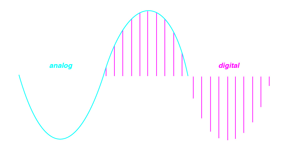
(Image by Janina Luckow)
This process comes with advantages and disadvantages, the main disadvantage being the loss of information between samples. During playback, this lost information is reconstructed during the digital to analog conversion process using a reconstruction filter. The advantage of digital representation, however, is that we may operate on the signal numerically and computationally.
Quantitative and Visual Descriptions of Sound in the Time Domain
Let’s return to figure 1.1 and discuss its properties in more detail. The horizontal dimension represents time, and the vertical dimension represents amplitude, a physical property related to the perceptual experience of loudness. This representation of a sound is said to be in the time domain, because it shows us how the signal varies as a function of time. We should keep in mind that what we experience as sound involves the higher-order cognitive processing of a dynamically changing 3-dimentional signal as it interacts with our environment over time. By contrast, figure 1.1 is a rather simple, two dimentional signal that can more accurately be thought of as the digitally sampled voltage of a transducer modulated over time by changes in air pressure at a particular location in space.
Let’s take a closer look at the details of a time-domain waveform.
Time Domain Representations of Signals
Frequency
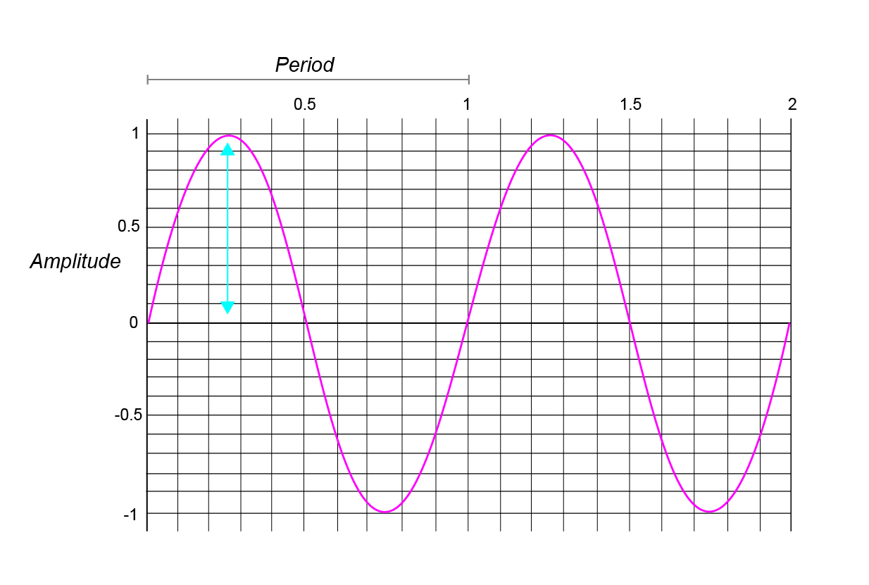
(Image by Janina Luckow)
In figure 1.5, we see a special waveform called a sine wave. A sine wave is special because it is periodic, meaning that its shape repeats over and over again. The amount of time it takes for it to repeat is called its period, and the number of periods that occur in one unit of time, say a second, is called its frequency. A sine wave is a plot of the position along the y-axis of a point as it travels counter-clockwise around a unit circle, starting from the point (1, 0).
(Animation by Janina Luckow)
As we mentioned above, the physical property amplitude is related to the perceptual experience of loudness. Additionally, the frequency of this sine wave is related to the perceptual experience of pitch, with higher frequencies and shorter periods correlating to higher sounding pitches, or notes.
Phase
The phase is the position in the period relative to some point that we determine to be the beginning. The phase tells us how much of the periodic waveform has elapsed, and consequently, how much will have to occur before the waveform repeats. Since phase is a representation of something that repeats or loops over and over again, we can think of it as a point traveling around a circle, and indeed, phase is usually represented as an angle expressed in degress ($0–360^{\circ}$) or in radians ($0–2\pi$).
A cosine wave appears exactly the same as a sine wave, shifted $1/4$ of a period to the left.
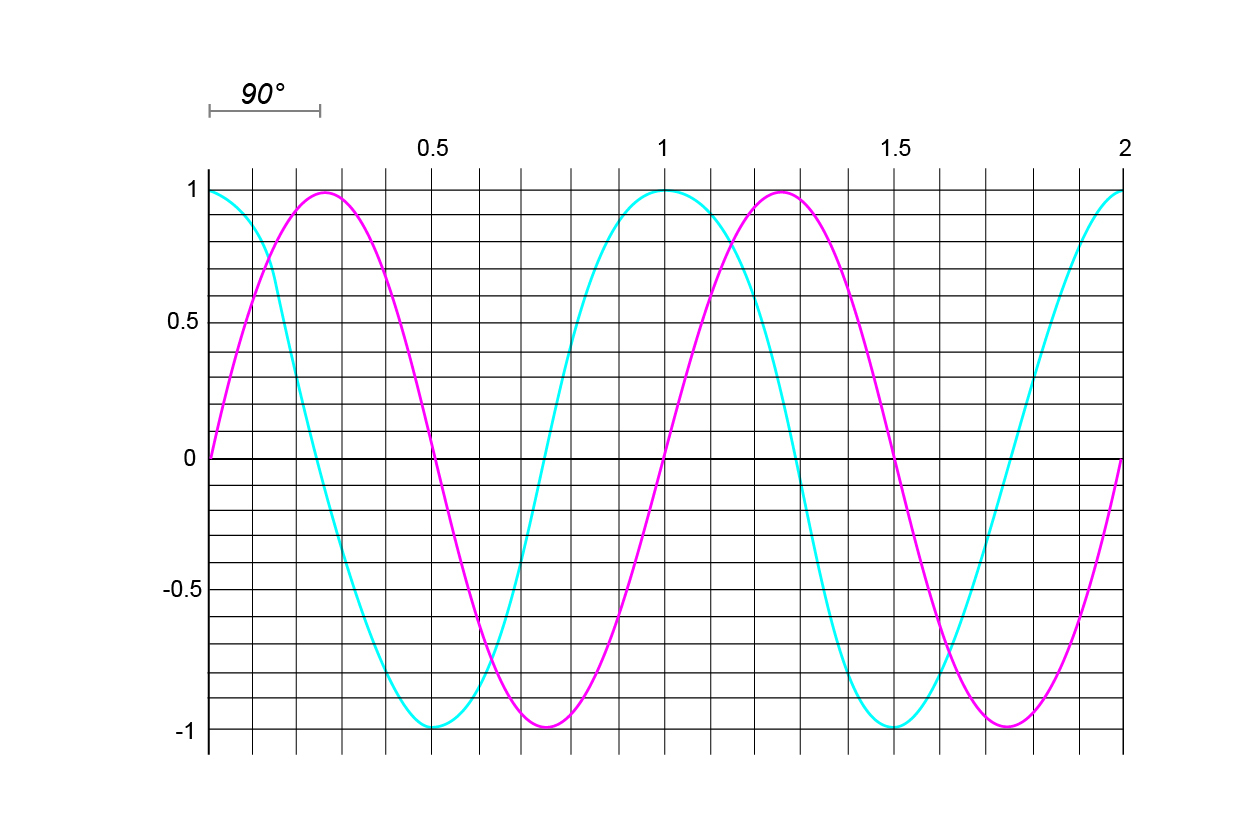
(Image by Janina Luckow)
Where a sine wave was the position along the y-axis, a cosine wave is the position of the same point along the x-axis.
(Animation by Janina Luckow)
Since the phase difference between a sine wave and a cosine wave is $1/4$ of a period, and that corresponds to our point having traveled $1/4$ of the way around the circle, or $90^{\circ}$, we can say that the two have a phase difference of $90^{\circ}$.
How Does Phase Affect Sound?
If a sine wave and a cosine wave are identical with the exception of a time shift, they should sound identical, right? Well they do. That doesn’t mean that phase isn’t important, but its affect on sound is not always intuitive. For a sinusoid by itself, it is impossible to hear any difference, no matter where it started in its cycle. Where you can begin to hear a difference is when you start to combine different sine waves.
When two sinusoids are added together, the relationship of their phase and frequency determines how they sound. When they have the same frequency and phase, the result is a sinusoid with an amplitude equal to the sum of the two. But when the phase of one of them is exactly half that of the other, the two cancel each other out and produce a flat waveform of 0 amplitude. Try shifting the phase of one sinusoid against another in the example below.
(Applet by John MacCallum)
You might notice a subtle change in pitch when you move the slider quickly— this is because a shift in phase requires the waveform to “jump” forward (or backward) faster (or slower) than it would have normally, and that change in the speed of the evolution of the waveform is a temporary change in frequency.
In the figure below we have a more complex example containing four sinusoids of different frequencies. The phases can be randomized, but the frequencies stay the same. Note that although the waveform changes dramatically when the phases change, the sound doesn’t change much. This is important, because it tells us that while the time-domain representation of a sound is certainly important, it does not often tell us much about how a signal will actually sound. Below, we will look at another representation of signals, the frequency-domain, but before that, let’s look at more complex waveforms.
| Gains: | Phases (0-360): |
(Applet by John MacCallum)
Summary
We have been looking at different representations of sounds, and before moving on, we should be clear how these relate to the physical phenomena they describe. The time-domain representation of a signal can be thought of as representing changes in intensity that propagate through some medium, and the path through different media from some event in the world to your brain is a complex one: objects collide to produce fluctuations in air pressure, which enter your ear and are transferred through bone, fluid, hair cells, and finally into the electrical signals of your nervous system. The 2-D drawings above could just as easily represent any of these, just as they could also represent the voltage as a function of time that moves a speaker cone back and forth (that produces changes in air pressure), the displacement of that speaker cone, etc.
Pure and Complex Sounds
So far, we have been looking at simple, “pure” waveforms, i.e. signals that can be characterized as having only a single frequency or pitch. When we add simple sounds together, as we did in figure 1.9, we produce complex sounds. The configuration of the different frequency components relative to one another account for much of the ways in which we experience timbre or the tone color of a sound, that is, the thing that makes a clarinet sound like a clarinet and a piano sound like a piano (more on this in the unit on timbre).
When pure tones with frequencies that are integer multiples of some frequency are added together, we say that they are in a harmonic relationship; all other sounds are said to be inharmonic. For example, if you had a tone that played at 440 cycles per second – the pitch concert A that many orchestras tune to– and added another tone that played at 880 cycles per second, this would create a harmonic relationship. If you instead added a tone the played at 457 cycles per second, this would be inharmonic.
In reality, all sounds are complex—there are no truely pure sounds. The sinusoids we discussed above are only theoretical, and any physical representation of them contains other frequency components, no matter how small, that distort their shape to some degree due to nonlinearities in the media that carry them. Consider air, for example, which is not at a uniform temperature and humidity everywhere. Since sound travels at a speed that is dependent upon temperature and humidity, small changes in the air produce small changes that manifest as distortion or noise.
Frequency Domain Representations of Signals
As we saw in figure 1.9, the time-domain representation of a signal is useful for certain things. For example, if you are editing some audio for a track you are working on in a digital audio workstation like Audacity, Garage Band, or ProTools, it makes sense to be able to “see” the waveform of the sound as it progresses over time.
From the amplitude of the wave you can see where it gets louder and depending on where you scroll on the wave you can find a specific point in the time of the track. But there is still a lot of information in that complex wave that might be useful.
What if we could take a wave form and suspend it in time, then look at a portion of it to get a better idea of all the component parts that make up the complex wave? In our next section, we look at a mathematical technique called Fourier transform that allows us to do just that.
Fourier Transform
We can move from the time-domain into the frequency-domain through a transformation of the signal known as the Fourier Transform, after Joseph Fourier. We’re going to take a brief dive into the math behind it, but don’t worry if it all doesn’t click on your first read. Wrapping your head around what the Fourier Transform is doing can be difficult, but once you understand it, it can be used as very powerful tool.
The Fourier Transform (FT) is a function that takes a time-domain signal as its input and produces a function of frequency as its output: \begin{equation} F(t)=\int_{-\infty}^{\infty}f(t)e^{-i2\pi xt}dt \label{eq:fouriertransform} \end{equation} where $f(t)$ is our time-domain function, and $F(t)$ is our frequency-domain function.
You might note those infinity signs above and below the integral symbol— indeed, from the perspective of the FT, a periodic signal can only be considered periodic if it is periodic forever! Since we can’t wait that long to compute the FT, we can use the Discrete Fourier Transform (DFT), which is a computation-friendly version of the continuous FT (sometimes you’ll hear people refer to the FFT which stands for the Fast Fourier Transform— this is simply a particular algorithm for computing the DFT):
\begin{equation} X(k)=\sum^{N-1}_{n=0}x(n)e^{-i2\pi\frac{kn}{N}} \label{eq:dft} \end{equation}
This may or may not look familiar, but just bear with me. $x(n)$ is our digitally-sampled time-domain signal, and $X(k)$ is the resulting frequency-domain representation of it. $e^{-i2\pi\frac{kn}{N}}$ can be rewritten using the (trigonometric) $\sin$ and $\cos$ functions: \begin{equation} e^{-i2\pi\frac{kn}{N}} = \cos\left(2\pi \frac{kn}{N}\right) - i \sin\left(2\pi \frac{kn}{N}\right) \label{eq:trig} \end{equation} So, when we rewrite the DFT in its less compact form: \begin{equation} X(k)=\sum^{N-1}_{n=0}x(n)\left[ \cos\left(2\pi \frac{kn}{N}\right) - i \sin\left(2\pi \frac{kn}{N}\right) \right] \label{eq:dft-trig} \end{equation} we can see that what the DFT is actually doing is multiplying our original signal by a bunch of sinusoids of different frequencies and summing the results, giving us a signal that tells us effectively “how much” of these frequencies the signal “contains”.
How many frequencies and which ones depends on that value $N$, and is up to you to decide, however, there is a tradeoff: the larger $N$ is, the more time it takes to collect those samples. While you get better frequency resolution when $N$ is large, you get poorer time resolution, and vice versa.
An important (and incredible) property of both the FT and the DFT is that they are reversible without any loss of information or change to the signal: you can convert fromthe time-domain to the frequency-domain and back and recover your original signal exactly. The inverse DFT (IDFT) looks remarkably similar to the DFT: \begin{equation} x(k)=\frac{1}{N}\sum^{N-1}_{n=0}X(n)e^{i2\pi\frac{kn}{N}} \label{eq:idft} \end{equation} (Note that the $X(n)$ and $x(n)$ are swapped relative to the DFT, by convention there is a $1/N$ normalization, and, if you missed it, there is a little missing “-“ sign in the exponent towards the right-hand side).
It can be difficult to form an intuition for the FT and DFT based on the equations alone. The following video provides a really nice visual demonstration of how this all works:
While that is probably more math than you might normally come into contact with in a course on music psychology, the FT allows us to perform very clever types of analyses of sounds as we will see below.
Spectrum
Once a waveform has been converted from the time domain to the frequency domain using a Fourier transformation, the resulting representation is often referred to as its spectrum. The spectrum is basically a snapshot of the component parts of whatever waveform that you fed into the Fourier transform. You could do this with something as short as a recording of a pluck of a single note on a banjo or an entire symphony.
(Audio by John MacCallum)
Looking at a sound’s spectrum, we now have a more clear view of the frequency composition of a signal. Although the DFT does actually produce the phase of each component, that information is often thrown away in the name of efficiency, which is also a tacit statement that it is a significantly less important feature than the frequency information.
Another representation of the spectrum over time is called a sonogram:
(Audio by John MacCallum)
Here, we can see a history of the spectrum over time, with the height representing frequency, the brightness magnitude (related to amplitude), and time along the x-axis.
The reason that we might want to make a sonogram is if we wanted to visually investigate the component parts of a sound. For example, above we learned that a sound’s timbre or tone color is partially determined by what combinations of wave forms make up the sound. Looking at the images below, we are unable to see anything distinct in the timbres of a short clip of a clarinet versus an oboe in the time domain.
|
| |
|
| |
Looking at these exact same clips of sound, but now in the frequency domain, we can see that the two sounds are very different. Inspecting these audio clips in the frequency domain allows us to see an audio fingerprint of each of the instrument’s timbres. Using spectrograms is only made possible with the Fourier transform and is the basis for investigating questions of musical timbre, automatic chord transcription, as well as many other tasks of musical analysis.
Links and Downloads
As part of MUTOR 2.0, the Multimedia Kontor Hamburg https://www.mmkh.de has developed a “Virtual Harp”, that may be played while wearing an Oculus Quest. Instructions for download and installation may be found here
Quiz
Briefly explain how a microphone works.
What is the term for the way in which energy moves between different media?
What were the two signal domains discussed?
What is the name of the process by which a signal is converted from one of these domains to the other?
Describe how time, frequency, and magnitude (amplitude) are represented in a sonogram.